Today unfortunetely one of the games best players and the current Bronwnlow Medalist Tom Mitchell has been injured and will probably miss the whole 2019 AFL season. This is horrible news as he was just coming off arguably his best season (winning the Brownlow Medal). He’s an incredibly gifted inside player who through the Hawks savvy recruiting have just gotten him some extra outside players to handball the ball too.
To put in perspective just how good of a season hes had, I thought I’d share some R script and hopefully some of you will have your own take on just how good of a season hes had and just what Hawthorn is missing in 2019.
Contested Possession King
Tom Mitchell we know is a contested possession machine, just how much of a machine was he?
One quick way would be just to see what is the average amount of contested possessions he got per game and where did that rank in terms of all the AFL players this year.
library(tidyverse)## ── Attaching packages ───────────────────────────────────────────────────────── tidyverse 1.2.1 ──## ✔ ggplot2 3.1.0 ✔ purrr 0.2.5
## ✔ tibble 2.0.1 ✔ dplyr 0.7.8
## ✔ tidyr 0.8.2 ✔ stringr 1.3.1
## ✔ readr 1.3.1 ✔ forcats 0.3.0## ── Conflicts ──────────────────────────────────────────────────────────── tidyverse_conflicts() ──
## ✖ dplyr::filter() masks stats::filter()
## ✖ dplyr::lag() masks stats::lag()fitzRoy::player_stats%>%
filter(Season==2018)%>%
group_by(Player)%>%
summarise(meanCP=mean(CP))%>%
arrange(desc(meanCP))## # A tibble: 657 x 2
## Player meanCP
## <chr> <dbl>
## 1 Patrick Cripps 17.6
## 2 Tom Mitchell 16.2
## 3 Clayton Oliver 16.2
## 4 Nathan Fyfe 16.1
## 5 Ben Cunnington 15.5
## 6 Patrick Dangerfield 15
## 7 Lachie Neale 15.0
## 8 Josh P. Kennedy 13.7
## 9 Jarryd Lyons 13.6
## 10 Jack Viney 13.5
## # … with 647 more rowsSo we can see here that he actually ranked second behind Patrick Cripps, but does that tell the whole story?
Supercoach King
I don’t mean this as what will Tom Mitchell missing be on your fantasy team, what I mean is Supercoach scores are probably the best measure of a good player that we have available in fitzRoy.
We know a few things about SC scores, we don’t know their actual formula that is some champion data secret sauce. But in general it does pass the eye test, good players get good scores. If you were to pick a SC team based only on scores it would probably look pretty good. We also know that on average a game will get to about 3300 which we can verify below.
library(tidyverse)
check<-fitzRoy::player_stats%>%
  group_by(Match_id)%>%
  summarise(sumSC=sum(SC))%>%
  arrange(desc(sumSC))
summary(check$sumSC)
## Min. 1st Qu. Median Mean 3rd Qu. Max.
## 3249 3299 3300 3300 3302 3331So we can see the mean and the median are the same.
Lets see how what % of supercoach scores does Tom Mitchell get per game on average and how does that compare?
fitzRoy::player_stats%>%
    group_by(Match_id)%>%
    mutate(pertSC=SC/sum(SC))%>%
    group_by(Season, Player)%>%
    summarise(mean=100*mean(pertSC))%>%
  arrange(desc(mean))
## # A tibble: 5,851 x 3
## # Groups: Season [9]
## Season Player mean
## <dbl> <chr> <dbl>
## 1 2012 Gary Jnr Ablett 4.19
## 2 2014 Gary Jnr Ablett 4.14
## 3 2017 Patrick Dangerfield 4.07
## 4 2014 Tom Rockliff 4.00
## 5 2016 Patrick Dangerfield 4.00
## 6 2010 Brendon Goddard 3.97
## 7 2018 Brodie Grundy 3.95
## 8 2011 Scott Pendlebury 3.93
## 9 2013 Gary Jnr Ablett 3.91
## 10 2018 Tom Mitchell 3.90
## # … with 5,841 more rowsBut just how good are these top 10 years? Lets look at it graphically.
fitzRoy::player_stats%>%
    group_by(Match_id)%>%
    mutate(pertSC=SC/sum(SC))%>%
    group_by(Season, Player)%>%
    summarise(mean=100*mean(pertSC))%>%
    ggplot(aes(x=mean))+geom_density() + geom_vline(xintercept = 3.90)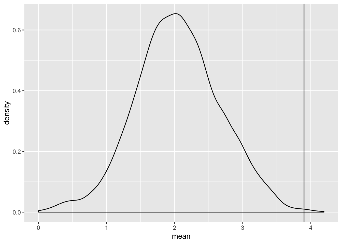
But thats since 2010, what about just in the 2018 season?
fitzRoy::player_stats%>%
        filter(Season==2018)%>%
      group_by(Match_id)%>%
    mutate(pertSC=SC/sum(SC))%>%
    group_by(Season, Player)%>%
    summarise(mean=100*mean(pertSC))%>%
  arrange(desc(mean))
## # A tibble: 657 x 3
## # Groups: Season [1]
## Season Player mean
## <dbl> <chr> <dbl>
## 1 2018 Brodie Grundy 3.95
## 2 2018 Tom Mitchell 3.90
## 3 2018 Jackson Macrae 3.85
## 4 2018 Max Gawn 3.78
## 5 2018 Patrick Dangerfield 3.63
## 6 2018 Patrick Cripps 3.62
## 7 2018 Nathan Fyfe 3.45
## 8 2018 Clayton Oliver 3.44
## 9 2018 Lachie Neale 3.39
## 10 2018 Jake Lloyd 3.35
## # … with 647 more rowsHere we can see Tom Mitchell ranks second, just behind Brodie Grundy.
Mitchells midfield impact
Max Laughton wrote a piece referencing stats provided from HPN about Tom Mitchells impact
Mitchell had 786 disposals over the 2018 home and away season; that was 9.4 per cent of Hawthorn’s team disposals total. Unsurprisingly, the next most reliant team was Carlton on Patrick Cripps; he had 652 disposals, 8.5 per cent of Carlton’s total disposal count. Cripps and Mitchell were the two most relied-upon midfielders in the AFL in 2018; Cripps had the largest proportion in the AFL of his team’s total contested possessions (13 per cent) and clearances (22.1 per cent), while Mitchell was second in those categories (11.3 and 21.5 per cent respectively)."
But I was left thinking I wonder how does that stack up as a percentage of the midfield group and what about the other teams? Do most teams have a high reliance on one midfielder? Are Cripps and Mitchell outliers or is this just a general footy thing?
You might also have an idea, maybe you don’t want to know about the clearances and the contested possessions and disposals. Perhaps you are interested in the % of score involvements, or club proportion of Brownlow Votes. These stats and a many others are in fitzRoy.
What I’m going to run through next, is just some ggplot visualisations of Tom Mitchells %s of Hawthorns midfield group with respect to a few things that were not covered in Max’s article. Specially looking at SC and score involvements. But we could also look at clearances, disposals and contested possessions because the data is there within fitzRoy.
You might have other ideas and that’s great hopefully you can take these scripts.
Lets now join on the player position data. There will be positional in data in fitzRoy it is on my to-do list I swear!
library(rvest)## Loading required package: xml2##
## Attaching package: 'rvest'## The following object is masked from 'package:purrr':
##
## pluck## The following object is masked from 'package:readr':
##
## guess_encodinglibrary(tidyverse)
library(stringr)
url<-"https://www.footywire.com/afl/footy/ft_players"
link<-read_html(url)%>%
html_nodes("br+ a , .lnormtop a:nth-child(1)")%>%
html_attr("href")
url_players<-str_c("https://www.footywire.com/afl/footy/",link)
cbind.fill <- function(...){
nm <- list(...)
nm <- lapply(nm, as.matrix)
n <- max(sapply(nm, nrow))
do.call(cbind, lapply(nm, function (x)
rbind(x, matrix(, n-nrow(x), ncol(x)))))
}
player_info <- function(x){
# page <- read_html(x)
page<-read_html(x)
player<- page%>%
html_nodes(".ldrow .hltitle")%>%
html_text() %>% as_tibble()
playing.for<- page%>%
html_nodes(".ldrow a b")%>%
html_text() %>% as_tibble()
number<- page%>%
html_nodes(".ldrow > b")%>%
html_text() %>% as_tibble()
weight<-page%>%
html_nodes("form tr:nth-child(4) .ldrow")%>%
html_text()%>%
str_replace_all("[\r\n]" , "")%>%
str_squish()%>%
str_extract(pattern =("(?<=Weight:).*(?=Position:)"))%>%as_tibble()
height<-page%>%
html_nodes("form tr:nth-child(4) .ldrow")%>%
html_text()%>%
str_replace_all("[\r\n]" , "")%>%
str_squish()%>%
str_extract(pattern =("(?<=Height:).*(?=Weight:)"))%>%as_tibble()
draft_position <- page%>%
html_nodes("tr:nth-child(5) .ldrow")%>%
html_text()%>%
str_replace_all("[\r\n]" , "")%>%
str_squish()%>%
str_extract(pattern =("(?<=Drafted: ).*(?=by)"))%>%as_tibble()
club_drafted <- page%>%
html_nodes("tr:nth-child(5) .ldrow")%>%
html_text()%>%str_replace_all("[\r\n]" , "")%>%
str_squish()%>%
str_remove(".*by") %>% as_tibble()
position <- page%>%
html_nodes("form tr:nth-child(4) .ldrow")%>%
html_text()%>%
str_replace_all("[\r\n]" , "")%>%
str_remove(".*Position: ")%>%
str_squish() %>% as_tibble()
#combine, name, and make it a tibble
player_information <- cbind.fill(player, playing.for, number, weight, height,draft_position, club_drafted, position)
player_information <- as_tibble(player_information)
# print(x)
# return(x)
return(player_information)
}
footywire <- purrr::map_df(url_players, player_info)## Warning: Calling `as_tibble()` on a vector is discouraged, because the behavior is likely to change in the future. Use `enframe(name = NULL)` instead.
## This warning is displayed once per session.## Warning: `as_tibble.matrix()` requires a matrix with column names or a `.name_repair` argument. Using compatibility `.name_repair`.
## This warning is displayed once per session.names(footywire) <- c("player", "club", "number","weight","height", "draft_position", "club_drafted", "position")
head(footywire)## # A tibble: 6 x 8
## player club number weight height draft_position club_drafted position
## <chr> <chr> <chr> <chr> <chr> <chr> <chr> <chr>
## 1 Jake A… Richm… #39 <NA> <NA> <NA> "" ""
## 2 Ryan A… Geelo… #45 " 100… " 200… Round 4, Pick … " Geelong C… Ruck
## 3 Gary J… Geelo… #4 " 87k… " 182… Round 3, Pick … " Geelong C… Midfield
## 4 Blake … St Ki… #8 " 92k… " 190… Round 1, Pick … " St Kilda … Midfiel…
## 5 Marcus… Brisb… #24 " 98k… " 192… Round 2, Pick … " Western B… Defender
## 6 Taylor… Colli… #13 " 83k… " 181… Round 1, Pick … " GWS Giant… Midfielddf<-fitzRoy::player_stats%>%
filter(Season==2018)
dataset<-left_join(df, footywire, by=c("Player"="player","Team"="club"))
head(dataset)## Date Season Round Venue Player Team Opposition
## 1 2018-03-22 2018 Round 1 MCG Dustin Martin Richmond Carlton
## 2 2018-03-22 2018 Round 1 MCG Trent Cotchin Richmond Carlton
## 3 2018-03-22 2018 Round 1 MCG Josh Caddy Richmond Carlton
## 4 2018-03-22 2018 Round 1 MCG Kamdyn Mcintosh Richmond Carlton
## 5 2018-03-22 2018 Round 1 MCG Jack Riewoldt Richmond Carlton
## 6 2018-03-22 2018 Round 1 MCG Brandon Ellis Richmond Carlton
## Status Match_id CP UP ED DE CM GA MI5 One.Percenters BO TOG K HB D M
## 1 Home 9514 17 15 23 71.9 2 2 2 1 0 87 20 12 32 5
## 2 Home 9514 13 12 15 62.5 0 2 1 1 0 81 14 10 24 2
## 3 Home 9514 11 10 14 73.7 1 0 2 0 1 80 13 6 19 5
## 4 Home 9514 3 15 11 57.9 0 0 1 1 1 69 19 0 19 5
## 5 Home 9514 5 14 12 66.7 1 2 5 1 0 96 12 6 18 7
## 6 Home 9514 3 14 13 72.2 0 0 0 0 2 79 11 7 18 3
## G B T HO GA1 I50 CL CG R50 FF FA AF SC CCL SCL SI MG TO ITC T5 number
## 1 1 3 1 0 2 6 6 3 0 1 1 110 139 4 2 13 567 5 2 0 <NA>
## 2 0 0 4 0 2 5 7 2 0 2 0 86 94 2 5 10 293 5 3 1 <NA>
## 3 3 2 2 0 0 8 4 2 0 5 0 99 84 3 1 6 424 2 1 0 <NA>
## 4 0 1 1 0 0 8 1 5 3 0 1 74 50 1 0 7 644 5 4 0 <NA>
## 5 4 2 1 0 2 6 0 2 0 1 0 100 101 0 0 13 322 3 1 0 <NA>
## 6 0 1 3 0 0 4 0 5 2 0 0 69 51 0 0 6 417 5 5 0 <NA>
## weight height draft_position club_drafted position
## 1 <NA> <NA> <NA> <NA> <NA>
## 2 <NA> <NA> <NA> <NA> <NA>
## 3 <NA> <NA> <NA> <NA> <NA>
## 4 <NA> <NA> <NA> <NA> <NA>
## 5 <NA> <NA> <NA> <NA> <NA>
## 6 <NA> <NA> <NA> <NA> <NA>What we can see here is that the join didn’t work, this is because if we look at the pages we are getting the data from. Have different team names which we can see if we click here and here so lets fix this up.
An altertive way to see if its different would be to check a few values that you are joining on like so.
unique(footywire$club)## [1] "Richmond Tigers" "Geelong Cats"
## [3] "St Kilda Saints" "Brisbane Lions"
## [5] "Collingwood Magpies" "West Coast Eagles"
## [7] "Gold Coast Suns" "North Melbourne Kangaroos"
## [9] "Sydney Swans" "Essendon Bombers"
## [11] "Port Adelaide Power" "Adelaide Crows"
## [13] "Melbourne Demons" "Fremantle Dockers"
## [15] "Hawthorn Hawks" "GWS Giants"
## [17] "Western Bulldogs" "Carlton Blues"unique(fitzRoy::player_stats$Team)## [1] "Richmond" "Carlton" "Geelong"
## [4] "Essendon" "Melbourne" "Hawthorn"
## [7] "Brisbane" "West Coast" "Sydney"
## [10] "St Kilda" "Port Adelaide" "North Melbourne"
## [13] "Western Bulldogs" "Collingwood" "Fremantle"
## [16] "Adelaide" "Gold Coast" "GWS"footywire <- footywire%>%
mutate(club=replace(club, club=="Richmond Tigers", "Richmond") )%>%
mutate(club=replace(club, club=="Geelong Cats", "Geelong"))%>%
mutate(club=replace(club, club== "St Kilda Saints", "St Kilda"))%>%
mutate(club=replace(club, club=="Brisbane Lions", "Brisbane"))%>%
mutate(club=replace(club, club=="Collingwood Mapies", "Collingwood"))%>%
mutate(club=replace(club, club=="West Coast Eagles", "West Coast"))%>%
mutate(club=replace(club, club=="Gold Coast Suns", "Gold Coast"))%>%
mutate(club=replace(club, club=="North Melbourne Kangaroos", "North Melbourne"))%>%
mutate(club=replace(club, club=="Sydney Swans", "Sydney"))%>%
mutate(club=replace(club, club=="Essendon Bombers", "Essendon"))%>%
mutate(club=replace(club, club=="Port Adelaide Power", "Port Adelaide"))%>%
mutate(club=replace(club, club=="Adelaide Crows", "Adelaide"))%>%
mutate(club=replace(club, club=="Melbourne Demons", "Melbourne"))%>%
mutate(club=replace(club, club=="Fremantle Dockers", "Fremantle"))%>%
mutate(club=replace(club, club=="Hawthorn Hawks", "Hawthorn"))%>%
mutate(club=replace(club, club=="GWS Giants", "GWS"))%>%
mutate(club=replace(club, club=="Carlton Blues", "Carlton"))%>%as.data.frame()
df<-fitzRoy::player_stats%>%
  filter(Season==2018)


dataset<-left_join(df, footywire, by=c("Player"="player","Team"="club"))
head(dataset)
## Date Season Round Venue Player Team Opposition
## 1 2018-03-22 2018 Round 1 MCG Dustin Martin Richmond Carlton
## 2 2018-03-22 2018 Round 1 MCG Trent Cotchin Richmond Carlton
## 3 2018-03-22 2018 Round 1 MCG Josh Caddy Richmond Carlton
## 4 2018-03-22 2018 Round 1 MCG Kamdyn Mcintosh Richmond Carlton
## 5 2018-03-22 2018 Round 1 MCG Jack Riewoldt Richmond Carlton
## 6 2018-03-22 2018 Round 1 MCG Brandon Ellis Richmond Carlton
## Status Match_id CP UP ED DE CM GA MI5 One.Percenters BO TOG K HB D M
## 1 Home 9514 17 15 23 71.9 2 2 2 1 0 87 20 12 32 5
## 2 Home 9514 13 12 15 62.5 0 2 1 1 0 81 14 10 24 2
## 3 Home 9514 11 10 14 73.7 1 0 2 0 1 80 13 6 19 5
## 4 Home 9514 3 15 11 57.9 0 0 1 1 1 69 19 0 19 5
## 5 Home 9514 5 14 12 66.7 1 2 5 1 0 96 12 6 18 7
## 6 Home 9514 3 14 13 72.2 0 0 0 0 2 79 11 7 18 3
## G B T HO GA1 I50 CL CG R50 FF FA AF SC CCL SCL SI MG TO ITC T5 number
## 1 1 3 1 0 2 6 6 3 0 1 1 110 139 4 2 13 567 5 2 0 #4
## 2 0 0 4 0 2 5 7 2 0 2 0 86 94 2 5 10 293 5 3 1 #9
## 3 3 2 2 0 0 8 4 2 0 5 0 99 84 3 1 6 424 2 1 0 #22
## 4 0 1 1 0 0 8 1 5 3 0 1 74 50 1 0 7 644 5 4 0 #33
## 5 4 2 1 0 2 6 0 2 0 1 0 100 101 0 0 13 322 3 1 0 #8
## 6 0 1 3 0 0 4 0 5 2 0 0 69 51 0 0 6 417 5 5 0 #5
## weight height draft_position club_drafted
## 1 92kg 187cm Round 1, Pick #3 2009 National Draft Richmond Tigers
## 2 85kg 185cm Round 1, Pick #2 2007 National Draft Richmond Tigers
## 3 88kg 186cm Round 1, Pick #7 2010 National Draft Gold Coast Suns
## 4 91kg 191cm Round 2, Pick #31 2012 National Draft Richmond Tigers
## 5 92kg 193cm Round 1, Pick #13 2006 National Draft Richmond Tigers
## 6 82kg 181cm Round 1, Pick #15 2011 National Draft Richmond Tigers
## position
## 1 Midfield
## 2 Midfield
## 3 Midfield, Forward
## 4 Defender, Midfield
## 5 Forward
## 6 DefenderWhy this happens is we can look at two players one retired and one current and if we look to where the team name sits, we can see the page structure is slightly different.
Now that we have the dataset there are a few caveats
- the scrape was done in the off season, so it doesn’t take into account players who retired they won’t have a position. Secondly players who have changed teams in the off season are already on their new teams page, so this won’t align.
This is annoying I know, so what we can do is view the NA’s to see if this is much of an issue.
new_DF <- dataset[is.na(dataset$position),]

NA_Players<-unique(new_DF$Player)
head(NA_Players)
## [1] "Reece Conca" "Corey Ellis" "Jed Lamb" "Aaron Mullett"
## [5] "Sam P-Seton" "Matthew Wright"So what we can see is that there are 114 players who have changed clubs or been delisted so aren’t in the intial scrape.
So what should we do?
My initial first thoughts are, scrape all the pages. But that would be pretty tedius/time consuming
So lets see if its mainly a problem due to our join i.e. trying to join on both player and team.
An easy way to check that would be to re-do our join, but this time only join on player.
dataset<-left_join(df, footywire, by=c("Player"="player"))

new_DF <- dataset[is.na(dataset$position),]

NA_Players<-unique(new_DF$Player)
So we can see that we can match a few more players, there will still be a Tom Lynch (but thankfully they are both forwards) issue but does this fix up most of our players? Well not really…..
Our list has been lowered, but on inspection we can see some interesting problems, lets take Will Hoskin-Elliot on his footywire profile page where we got his details from (position), his name is listed as Will-Hoskin Elliott, but if we were to look at his in game statistics such as the afl grand final 2018 we can see that his name is listed as Will-H Elliott.
Isn’t that annoying!
So this is where some domain knowledge comes in handy, I am going to go through the above list and just manually encode those players I know are midfielders.
- Obviously I will miss a few
- I will probably misclassify a few too.
But I think for blogging purposes its good to see an example of a common problem like this and possible ways to fix it.
The longer, more robust way would be to scrape not only the current players, but the past players as well this will capture the retirees.
So how do we replace values?
dataset <- dataset %>%
  mutate(position = replace(position, which(is.na(position) &
                                          Player == "Sam P-Seton"), "Midfield, Forward"))%>%
  mutate(position = replace(position, which(is.na(position) &
                                          Player=="Brendon Goddard"), "Defender, Midfield"))%>%
  mutate(position = replace(position, which(is.na(position) &
                                          Player=="Cameron E-Yolmen"), "Midfield"))%>%
  mutate(position = replace(position, which(is.na(position) &
                                          Player=="Curtly Hampton"),"Midfield"))%>%
  mutate(position = replace(position, which(is.na(position) &
                                              Player=="Koby Stevens"),"Midfield"))%>%
  mutate(position = replace(position, which(is.na(position) &
                                              Player=="Dom Barry"),"Midfield"))%>%
  mutate(position = replace(position, which(is.na(position) &
                                              Player=="Sam P-Pepper"),"Midfield"))%>%
  mutate(position = replace(position, which(is.na(position) &
                                              Player=="Danyle Pearce"),"Forward"))%>%
  mutate(position = replace(position, which(is.na(position) &
                                              Player=="Matthew Rosa"),"Midfield"))%>%
  mutate(position = replace(position, which(is.na(position) &
                                              Player=="Billy Hartung"),"Midfield"))%>%
  mutate(position = replace(position, which(is.na(position) &
                                              Player=="Ed V-Willis"),"Defender"))%>%
  mutate(position = replace(position, which(is.na(position) &
                                              Player=="Jarrad Waite"),"Forward"))%>%
  mutate(position = replace(position, which(is.na(position) &
                                              Player=="Luke D-Uniacke"),"Midfield"))%>%
  mutate(position = replace(position, which(is.na(position) &
                                              Player=="Cyril Rioli"),"Forward"))%>%
  mutate(position = replace(position, which(is.na(position) &
                                              Player == "Will H-Elliott"), "Midfield, Forward"))%>%
  mutate(position = replace(position, which(is.na(position) &
                                              Player=="Shane Biggs"),"Defender"))%>%
  mutate(position = replace(position, which(is.na(position) &
                                              Player=="Mitch Honeychurch"),"Forward"))%>%
  mutate(position = replace(position, which(is.na(position) &
                                              Player=="Bernie Vince"),"Defender"))%>%
  mutate(position = replace(position, which(is.na(position) &
                                              Player=="Cameron Pedersen"),"Forward, Ruck"))%>%
  mutate(position = replace(position, which(is.na(position) &
                                              Player=="Alex N-Bullen"),"Forward"))%>%
  mutate(position = replace(position, which(is.na(position) &
                                              Player=="Cory Gregson"),"Forward"))%>%
  mutate(position = replace(position, which(is.na(position) &
                                              Player=="Mark Lecras"),"Forward"))%>%
  mutate(position = replace(position, which(is.na(position) &
                                              Player=="Dean Towers"),"Forward"))%>%
  mutate(position = replace(position, which(is.na(position) &
                                              Player=="Cameron O'Shea"),"Defender"))%>%
  mutate(position = replace(position, which(is.na(position) &
                                              Player == "Rohan Bewick"), "Midfield, Forward"))%>%
  mutate(position = replace(position, which(is.na(position) &
                                              Player=="Nathan Wright"),"Forward"))%>%
  mutate(position = replace(position, which(is.na(position) &
                                              Player=="Jack Redpath"),"Forward"))%>%
  mutate(position = replace(position, which(is.na(position) &
                                              Player=="Ryan Griffen"),"Midfield, Forward"))%>%
  mutate(position = replace(position, which(is.na(position) &
                                              Player=="Nicholas Graham"),"Midfield, Forward"))%>%
  mutate(position = replace(position, which(is.na(position) &
                                              Player=="Sam Gilbert"),"Defender"))%>%
  mutate(position = replace(position, which(is.na(position) &
                                              Player=="Harrison Marsh"),"Defender"))%>%
  mutate(position = replace(position, which(is.na(position) &
                                              Player==" Sam Kerridge"),"Midfield"))%>%
  mutate(position = replace(position, which(is.na(position) &
                                              Player=="Sam Rowe"),"Defender"))%>%
  mutate(position = replace(position, which(is.na(position) &
                                              Player=="Jake Neade"),"Forward"))%>%
  mutate(position = replace(position, which(is.na(position) &
                                              Player=="Lindsay Thomas"),"Forward"))%>%
  mutate(position = replace(position, which(is.na(position) &
                                              Player=="George H-Smith"),"Midfield"))%>%
  mutate(position = replace(position, which(is.na(position) &
                                              Player=="Jesse Lonergan"),"Midfield"))%>%
  mutate(position = replace(position, which(is.na(position) &
                                              Player=="Jackson Merrett"),"Defender, Forward"))%>%
  mutate(position = replace(position, which(is.na(position) &
                                              Player=="Daniel Robinson"),"Forward"))%>%
  mutate(position = replace(position, which(is.na(position) &
                                              Player=="Michael Barlow"),"Midfield, Forward"))%>%
  mutate(position = replace(position, which(is.na(position) &
                                              Player=="Max Spencer"),"Defender"))%>%
  mutate(position = replace(position, which(is.na(position) &
                                              Player=="Matthew Leuenberger"),"Ruck"))%>%
  mutate(position = replace(position, which(is.na(position) &
                                              Player=="Jarryd Blair"),"Forward"))%>%
  mutate(position = replace(position, which(is.na(position) &
                                              Player=="Stewart Crameri"),"Forward"))%>%
  mutate(position = replace(position, which(is.na(position) &
                                              Player=="Brad Scheer"),"Forward"))%>%
  mutate(position = replace(position, which(is.na(position) &
                                              Player=="Brendan Whitecross"),"Forward"))%>%
  mutate(position = replace(position, which(is.na(position) &
                                              Player=="Sam Gibson"),"Midfield"))%>%
  mutate(position = replace(position, which(is.na(position) &
                                              Player=="Tim Mohr"),"Defender"))%>%
  mutate(position = replace(position, which(is.na(position) &
                                              Player=="Aaron Black"),"Forward"))%>%
  mutate(position = replace(position, which(is.na(position) &
                                              Player=="Michael Apeness"),"Forward, Ruck"))%>%
  mutate(position = replace(position, which(is.na(position) &
                                              Player=="Kyle Cheney"),"Defender"))%>%
  mutate(position = replace(position, which(is.na(position) &
                                              Player=="Jake Barrett"),"Forward"))%>%
  mutate(position = replace(position, which(is.na(position) &
                                              Player=="Jonathan O'Rourke"),"Midfield"))%>%
  mutate(position = replace(position, which(is.na(position) &
                                              Player=="Matt Shaw"),"Midfield"))%>%
  mutate(position = replace(position, which(is.na(position) &
                                              Player=="Jay K-Harris"),"Midfield"))%>%
  mutate(position = replace(position, which(is.na(position) &
                                              Player=="Alex Morgan"),"Defender"))%>%
  mutate(position = replace(position, which(is.na(position) &
                                              Player=="Nathan Freeman"),"Midfield"))%>%
  mutate(position = replace(position, which(is.na(position) &
                                              Player=="Alex Johnson"),"Defender"))%>%
  mutate(position = replace(position, which(is.na(position) &
                                              Player=="Brady Grey"),"Forward"))%>%

  mutate(position = replace(position, which(is.na(position) &
                                              Player=="Adam Oxley"),"Defender"))
Now we have most of the players positions filled out, so now lets look at Tom Mitchells percentages as part of the midfield group.
Tom Mitchells contested possessions % as a midfield group
So I will define and this is of course up for debate as midfield group as plays in one of the following listed footywire positions. * Midfield * Midfield, Forward * Defender, Midfield, * Ruck, * Forward, Ruck
  dataset%>%
    filter(position %in% c("Midfield, Forward", "Midfield","Defender, Midfield", "Ruck", "Forward, Ruck"))%>%
    group_by(Team, Round)%>%
    summarise(sumCP=sum(CP))%>%
    group_by(Team)%>%
    summarise(meanCP=mean(sumCP))%>%
    arrange(desc(meanCP))
## # A tibble: 18 x 2
## Team meanCP
## <chr> <dbl>
## 1 Geelong 104.
## 2 Melbourne 101.
## 3 Collingwood 94.3
## 4 Port Adelaide 93.8
## 5 Brisbane 91.1
## 6 Adelaide 89.1
## 7 Western Bulldogs 87.6
## 8 Fremantle 86.6
## 9 North Melbourne 84.2
## 10 Richmond 83.7
## 11 Gold Coast 81.3
## 12 Essendon 81.2
## 13 Carlton 80.8
## 14 GWS 80.4
## 15 Sydney 79.3
## 16 West Coast 78.1
## 17 St Kilda 70.8
## 18 Hawthorn 68.4But how much does Tom Mitchell average by himself?
dataset%>%
    filter(position %in% c("Midfield, Forward", "Midfield","Defender, Midfield", "Ruck", "Forward, Ruck"))%>%
    group_by(Team, Round, Player)%>%
    summarise(sumCP=sum(CP))%>%
    group_by(Team, Player)%>%
    summarise(meanCP=mean(sumCP))%>%
    arrange(desc(meanCP))
## # A tibble: 301 x 3
## # Groups: Team [18]
## Team Player meanCP
## <chr> <chr> <dbl>
## 1 Carlton Patrick Cripps 17.6
## 2 Hawthorn Tom Mitchell 16.2
## 3 Melbourne Clayton Oliver 16.2
## 4 Fremantle Nathan Fyfe 16.1
## 5 North Melbourne Ben Cunnington 15.5
## 6 Geelong Patrick Dangerfield 15
## 7 Fremantle Lachie Neale 15.0
## 8 Sydney Josh P. Kennedy 13.7
## 9 Gold Coast Jarryd Lyons 13.6
## 10 Melbourne Jack Viney 13.5
## # … with 291 more rowsInterestingly Tom Mitchell averaged the second most contested possessions per game on the team that averaged in the bottom half of contested possessions (13) per week. Based on a first glance it seems pretty important.
To check the above statement we can use the script below
library(tidyverse)
fitzRoy::player_stats%>%
  filter(Season==2018)%>%
  group_by(Player, Team)%>%
  summarise(meanCP=mean(CP))%>%
  arrange(desc(meanCP))
## # A tibble: 658 x 3
## # Groups: Player [657]
## Player Team meanCP
## <chr> <chr> <dbl>
## 1 Patrick Cripps Carlton 17.6
## 2 Tom Mitchell Hawthorn 16.2
## 3 Clayton Oliver Melbourne 16.2
## 4 Nathan Fyfe Fremantle 16.1
## 5 Ben Cunnington North Melbourne 15.5
## 6 Patrick Dangerfield Geelong 15
## 7 Lachie Neale Fremantle 15.0
## 8 Josh P. Kennedy Sydney 13.7
## 9 Jarryd Lyons Gold Coast 13.6
## 10 Jack Viney Melbourne 13.5
## # … with 648 more rowsfitzRoy::player_stats%>%
filter(Season==2018)%>%
group_by(Team, Round)%>%
summarise(sumCP=sum(CP))%>%
group_by(Team)%>%
summarise(meanCP=mean(sumCP))%>%
arrange(desc(meanCP))## # A tibble: 18 x 2
## Team meanCP
## <chr> <dbl>
## 1 Melbourne 160
## 2 Adelaide 154.
## 3 Collingwood 153.
## 4 Geelong 150.
## 5 GWS 150.
## 6 Port Adelaide 149.
## 7 North Melbourne 149.
## 8 Richmond 148.
## 9 Sydney 147
## 10 Gold Coast 144.
## 11 West Coast 144.
## 12 Essendon 143.
## 13 Hawthorn 142.
## 14 Western Bulldogs 139.
## 15 Brisbane 136.
## 16 Fremantle 136.
## 17 Carlton 136.
## 18 St Kilda 136.We can then break that up a bit futher and look at just the teams midfield groups, this is where Tom Mitchells contribution becomes more obvious, Hawthorn actually are last in their midfields average contested possessions. Again we can verify that with the script below.
teamstats<-dataset%>%

  filter(position %in% c("Midfield, Forward", "Midfield","Defender, Midfield", "Ruck", "Forward, Ruck"))%>%
  group_by(Team, Round)%>%
  summarise(sumCP=sum(CP))%>%
  group_by(Team)%>%
  summarise(meanCPTeam=mean(sumCP))

teamstats%>%arrange(desc(meanCPTeam))
## # A tibble: 18 x 2
## Team meanCPTeam
## <chr> <dbl>
## 1 Geelong 104.
## 2 Melbourne 101.
## 3 Collingwood 94.3
## 4 Port Adelaide 93.8
## 5 Brisbane 91.1
## 6 Adelaide 89.1
## 7 Western Bulldogs 87.6
## 8 Fremantle 86.6
## 9 North Melbourne 84.2
## 10 Richmond 83.7
## 11 Gold Coast 81.3
## 12 Essendon 81.2
## 13 Carlton 80.8
## 14 GWS 80.4
## 15 Sydney 79.3
## 16 West Coast 78.1
## 17 St Kilda 70.8
## 18 Hawthorn 68.4So that Tom Mitchell, he ranks second in terms of average contested possessions per game in the midfield that gets the least amount of contested possessions per game.
But lets get back to what I wanted to look at earlier. That was specifically Tom Mitchells contribution as part of the midfield group.
teamstats<-dataset%>%

  filter(position %in% c("Midfield, Forward", "Midfield","Defender, Midfield", "Ruck", "Forward, Ruck"))%>%
  group_by(Team, Round)%>%
  summarise(sumCP=sum(CP))%>%
  group_by(Team)%>%
  summarise(meanCPTeam=mean(sumCP))


playerstats<-dataset%>%
  filter(position %in% c("Midfield, Forward", "Midfield","Defender, Midfield", "Ruck", "Forward, Ruck"))%>%
  group_by(Team, Round, Player)%>%
  summarise(sumCP=sum(CP))%>%
  group_by(Team, Player)%>%
  summarise(meanCPlayer=mean(sumCP))

df<-left_join(playerstats,teamstats , by=c("Team","Team"))%>%
  mutate(pertcontribution=meanCPlayer/meanCPTeam)

df%>%arrange(desc(pertcontribution))%>%head()
## # A tibble: 6 x 5
## # Groups: Team [5]
## Team Player meanCPlayer meanCPTeam pertcontribution
## <chr> <chr> <dbl> <dbl> <dbl>
## 1 Hawthorn Tom Mitchell 16.2 68.4 0.237
## 2 Carlton Patrick Cripps 17.6 80.8 0.218
## 3 Fremantle Nathan Fyfe 16.1 86.6 0.186
## 4 North Melbourne Ben Cunnington 15.5 84.2 0.184
## 5 Fremantle Lachie Neale 15.0 86.6 0.173
## 6 Sydney Josh P. Kennedy 13.7 79.3 0.172Looking at it this way, what could be an interesting observation Tom Mitchell averages less contested possessions per game, and less of a proportion of his teams contested possessions when comparing him vs Patrick Cripps. But if we were to just look as part of the teams midfield group. Tom Mitchell leads the league in terms of proportion of contested possessions won as part of the teams midfield.
Lets now have a quick look at this graphically. ;
df%>%
  ggplot(aes(x=as.factor(Team), y=pertcontribution))+
  geom_point(aes(colour=Team)) + theme(axis.text.x =
                                         element_text(angle = 90, hjust = 1)) +xlab("Team") +ylab("Proportion of Teams Midfield Groups Contested Posessions") + theme(legend.position="none")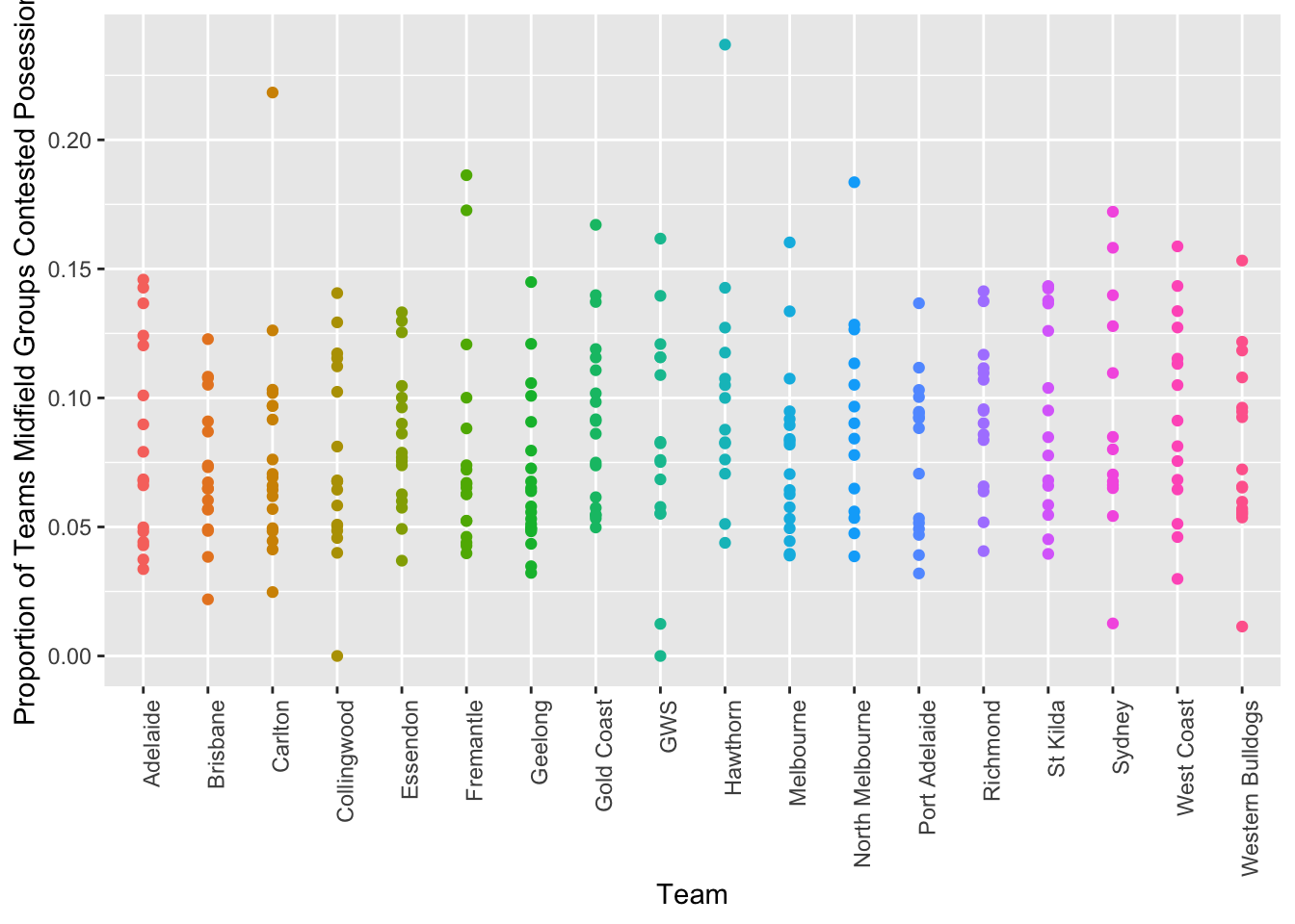
Tom Mitchells SC score %
teamstats<-dataset%>%

  filter(position %in% c("Midfield, Forward", "Midfield","Defender, Midfield", "Ruck", "Forward, Ruck"))%>%
  group_by(Team, Round)%>%
  summarise(sumSC=sum(SC))%>%
  group_by(Team)%>%
  summarise(meanSCTeam=mean(sumSC))


playerstats<-dataset%>%
  filter(position %in% c("Midfield, Forward", "Midfield","Defender, Midfield", "Ruck", "Forward, Ruck"))%>%
  group_by(Team, Round, Player)%>%
  summarise(sumSC=sum(SC))%>%
  group_by(Team, Player)%>%
  summarise(meanSClayer=mean(sumSC))

df<-left_join(playerstats,teamstats , by=c("Team","Team"))%>%
  mutate(pertcontribution=meanSClayer/meanSCTeam)

df%>%arrange(desc(pertcontribution))%>%head()
## # A tibble: 6 x 5
## # Groups: Team [5]
## Team Player meanSClayer meanSCTeam pertcontribution
## <chr> <chr> <dbl> <dbl> <dbl>
## 1 Hawthorn Tom Mitchell 129. 744. 0.173
## 2 Carlton Patrick Cripps 119. 792 0.151
## 3 St Kilda Sebastian Ross 103. 746. 0.138
## 4 Sydney Luke Parker 102. 744. 0.137
## 5 West Coast Andrew Gaff 108. 791. 0.137
## 6 Hawthorn Ben McEvoy 101. 744. 0.136df%>%ggplot(aes(x=as.factor(Team), y=pertcontribution))+geom_point(aes(colour=Team))+ theme(axis.text.x = element_text(angle = 90, hjust = 1))+xlab("Team") + theme(legend.position="none")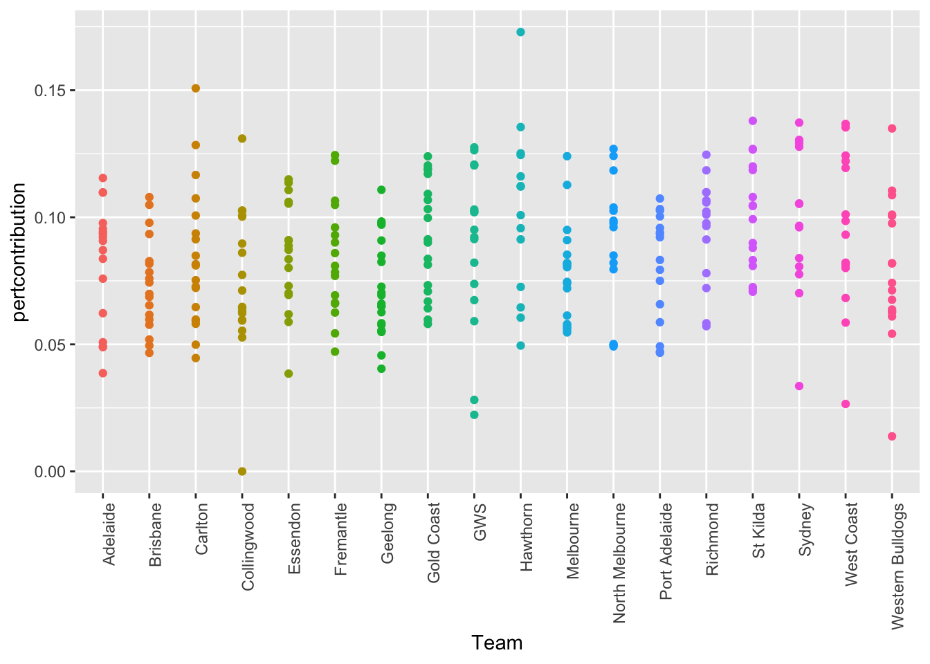
Tom Mitchell Score involvements
teamstats<-dataset%>%

  filter(position %in% c("Midfield, Forward", "Midfield","Defender, Midfield", "Ruck", "Forward, Ruck"))%>%
  group_by(Team, Round)%>%
  summarise(sumSI=sum(SI))%>%
  group_by(Team)%>%
  summarise(meanSITeam=mean(sumSI))


playerstats<-dataset%>%
  filter(position %in% c("Midfield, Forward", "Midfield","Defender, Midfield", "Ruck", "Forward, Ruck"))%>%
  group_by(Team, Round, Player)%>%
  summarise(sumSI=sum(SI))%>%
  group_by(Team, Player)%>%
  summarise(meanSIlayer=mean(sumSI))

df<-left_join(playerstats,teamstats , by=c("Team","Team"))%>%
  mutate(pertcontribution=meanSIlayer/meanSITeam)

df%>%arrange(desc(pertcontribution))
## # A tibble: 301 x 5
## # Groups: Team [18]
## Team Player meanSIlayer meanSITeam pertcontribution
## <chr> <chr> <dbl> <dbl> <dbl>
## 1 North Melbourne Shaun Higgins 7.25 47.0 0.154
## 2 Richmond Dustin Martin 8.57 55.8 0.154
## 3 Gold Coast Michael Barlow 4.67 30.5 0.153
## 4 Hawthorn Tom Mitchell 6.21 40.9 0.152
## 5 Fremantle Nathan Fyfe 7.93 52.4 0.151
## 6 Gold Coast Jarryd Lyons 4.47 30.5 0.147
## 7 West Coast Andrew Gaff 6.53 45.6 0.143
## 8 Hawthorn Jaeger O'Meara 5.71 40.9 0.140
## 9 Carlton Patrick Cripps 5.41 38.7 0.140
## 10 West Coast Luke Shuey 6.25 45.6 0.137
## # … with 291 more rowsdf%>%ggplot(aes(x=as.factor(Team), y=pertcontribution))+geom_point(aes(colour=Team))+ theme(axis.text.x = element_text(angle = 90, hjust = 1)) +xlab("Team") + theme(legend.position="none")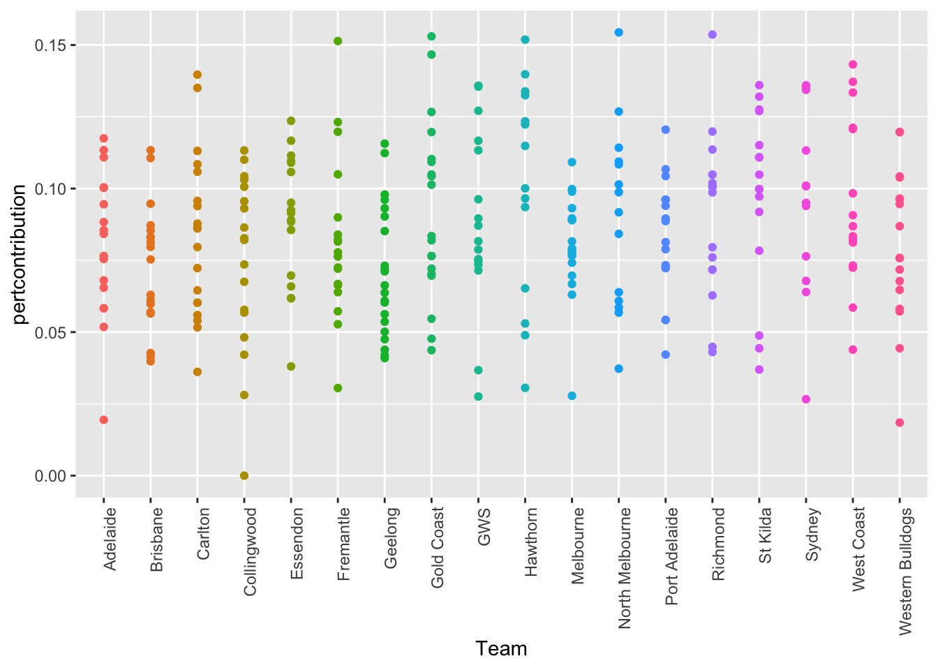
The score involvements is pretty interesting.
If we were to just look at average score involvements per game where do you think Tom Mitchell would rank?
Not even in the top 50, but his proportion of score involvements as a proportion of the Hawthorns midfield group is top 4.
So hopefully reading this has given you the itch to do some of your own analysis and putting your thoughts/ideas down and seeing if they come out in the data.
Tom Mitchell what a season.