One of the things I have always wondered about AFL fantasy is just who is the best fantasy player of all time? Not the fan who wins the most but who is the best player.
So one possible idea would be to work out the fantasy scores of players going back for all the time that is possible (YAY fitzRoy!). From there, lets look at the z-score of players in the individual year look at a plot for all years we have fantasy available and do some exploration.
Step One - Work out Fantasy Scores
library(tidyverse)## ── Attaching packages ─────────────────────────────────────────────────────────────────────── tidyverse 1.2.1 ──## ✔ ggplot2 3.1.0 ✔ purrr 0.3.2
## ✔ tibble 2.1.1 ✔ dplyr 0.8.0.1
## ✔ tidyr 0.8.3 ✔ stringr 1.4.0
## ✔ readr 1.3.1 ✔ forcats 0.4.0## ── Conflicts ────────────────────────────────────────────────────────────────────────── tidyverse_conflicts() ──
## ✖ dplyr::filter() masks stats::filter()
## ✖ dplyr::lag() masks stats::lag()df<-fitzRoy::get_afltables_stats(start_date="1987-01-01", end_date = "2018-10-10")%>%
mutate(AF=3*Kicks + 2*Handballs + 3*Marks +
4*Tackles+ Frees.For -
3*Frees.Against +Hit.Outs+
6*Goals +Behinds)## Returning data from 1987-01-01 to 2018-10-10## Downloading data##
## Finished downloading data. Processing XMLs## Warning: Detecting old grouped_df format, replacing `vars` attribute by
## `groups`## Finished getting afltables dataOnce we have worked out the fantasy scores we need to come up with our filters and our groups with of course sensible checks and balances.
We know that tackles first started getting recorded in 1987, so lets filter our dataset by Season> 1986
df%>%

  filter(Season>1986)
## # A tibble: 254,507 x 60
## Season Round Date Local.start.time Venue Attendance Home.team
## <dbl> <chr> <date> <int> <chr> <int> <chr>
## 1 1991 1 1991-03-22 1940 Foot… 44902 Adelaide
## 2 1991 1 1991-03-22 1940 Foot… 44902 Adelaide
## 3 1991 1 1991-03-22 1940 Foot… 44902 Adelaide
## 4 1991 1 1991-03-22 1940 Foot… 44902 Adelaide
## 5 1991 1 1991-03-22 1940 Foot… 44902 Adelaide
## 6 1991 1 1991-03-22 1940 Foot… 44902 Adelaide
## 7 1991 1 1991-03-22 1940 Foot… 44902 Adelaide
## 8 1991 1 1991-03-22 1940 Foot… 44902 Adelaide
## 9 1991 1 1991-03-22 1940 Foot… 44902 Adelaide
## 10 1991 1 1991-03-22 1940 Foot… 44902 Adelaide
## # … with 254,497 more rows, and 53 more variables: HQ1G <int>, HQ1B <int>,
## # HQ2G <int>, HQ2B <int>, HQ3G <int>, HQ3B <int>, HQ4G <int>,
## # HQ4B <int>, Home.score <int>, Away.team <chr>, AQ1G <int>, AQ1B <int>,
## # AQ2G <int>, AQ2B <int>, AQ3G <int>, AQ3B <int>, AQ4G <int>,
## # AQ4B <int>, Away.score <int>, First.name <chr>, Surname <chr>,
## # ID <dbl>, Jumper.No. <dbl>, Playing.for <chr>, Kicks <dbl>,
## # Marks <dbl>, Handballs <dbl>, Goals <dbl>, Behinds <dbl>,
## # Hit.Outs <dbl>, Tackles <dbl>, Rebounds <dbl>, Inside.50s <dbl>,
## # Clearances <dbl>, Clangers <dbl>, Frees.For <dbl>,
## # Frees.Against <dbl>, Brownlow.Votes <dbl>,
## # Contested.Possessions <dbl>, Uncontested.Possessions <dbl>,
## # Contested.Marks <dbl>, Marks.Inside.50 <dbl>, One.Percenters <dbl>,
## # Bounces <dbl>, Goal.Assists <dbl>, Time.on.Ground.. <int>,
## # Substitute <int>, Umpire.1 <chr>, Umpire.2 <chr>, Umpire.3 <chr>,
## # Umpire.4 <chr>, group_id <int>, AF <dbl>Our next stage, we are going to add a count of the games each player played in during the Season, we make this decision because we want to have a look at players who had the best season, not just the best games and 10 seems like a reasonable cut off
df%>%
  filter(Season>1986)%>%
  group_by(Season, ID)%>%
  mutate(countgames=n())
## # A tibble: 254,507 x 61
## # Groups: Season, ID [18,678]
## Season Round Date Local.start.time Venue Attendance Home.team
## <dbl> <chr> <date> <int> <chr> <int> <chr>
## 1 1991 1 1991-03-22 1940 Foot… 44902 Adelaide
## 2 1991 1 1991-03-22 1940 Foot… 44902 Adelaide
## 3 1991 1 1991-03-22 1940 Foot… 44902 Adelaide
## 4 1991 1 1991-03-22 1940 Foot… 44902 Adelaide
## 5 1991 1 1991-03-22 1940 Foot… 44902 Adelaide
## 6 1991 1 1991-03-22 1940 Foot… 44902 Adelaide
## 7 1991 1 1991-03-22 1940 Foot… 44902 Adelaide
## 8 1991 1 1991-03-22 1940 Foot… 44902 Adelaide
## 9 1991 1 1991-03-22 1940 Foot… 44902 Adelaide
## 10 1991 1 1991-03-22 1940 Foot… 44902 Adelaide
## # … with 254,497 more rows, and 54 more variables: HQ1G <int>, HQ1B <int>,
## # HQ2G <int>, HQ2B <int>, HQ3G <int>, HQ3B <int>, HQ4G <int>,
## # HQ4B <int>, Home.score <int>, Away.team <chr>, AQ1G <int>, AQ1B <int>,
## # AQ2G <int>, AQ2B <int>, AQ3G <int>, AQ3B <int>, AQ4G <int>,
## # AQ4B <int>, Away.score <int>, First.name <chr>, Surname <chr>,
## # ID <dbl>, Jumper.No. <dbl>, Playing.for <chr>, Kicks <dbl>,
## # Marks <dbl>, Handballs <dbl>, Goals <dbl>, Behinds <dbl>,
## # Hit.Outs <dbl>, Tackles <dbl>, Rebounds <dbl>, Inside.50s <dbl>,
## # Clearances <dbl>, Clangers <dbl>, Frees.For <dbl>,
## # Frees.Against <dbl>, Brownlow.Votes <dbl>,
## # Contested.Possessions <dbl>, Uncontested.Possessions <dbl>,
## # Contested.Marks <dbl>, Marks.Inside.50 <dbl>, One.Percenters <dbl>,
## # Bounces <dbl>, Goal.Assists <dbl>, Time.on.Ground.. <int>,
## # Substitute <int>, Umpire.1 <chr>, Umpire.2 <chr>, Umpire.3 <chr>,
## # Umpire.4 <chr>, group_id <int>, AF <dbl>, countgames <int>Our next stage is that we want to work out the z-scores of the fantasy players per game by by season
df%>%
  filter(Season>1986)%>%
  group_by(Season, ID)%>%
  mutate(countgames=n())%>%
  group_by(Season)%>%
  mutate(Z_score=(AF-mean(AF))/sd(AF))
## # A tibble: 254,507 x 62
## # Groups: Season [32]
## Season Round Date Local.start.time Venue Attendance Home.team
## <dbl> <chr> <date> <int> <chr> <int> <chr>
## 1 1991 1 1991-03-22 1940 Foot… 44902 Adelaide
## 2 1991 1 1991-03-22 1940 Foot… 44902 Adelaide
## 3 1991 1 1991-03-22 1940 Foot… 44902 Adelaide
## 4 1991 1 1991-03-22 1940 Foot… 44902 Adelaide
## 5 1991 1 1991-03-22 1940 Foot… 44902 Adelaide
## 6 1991 1 1991-03-22 1940 Foot… 44902 Adelaide
## 7 1991 1 1991-03-22 1940 Foot… 44902 Adelaide
## 8 1991 1 1991-03-22 1940 Foot… 44902 Adelaide
## 9 1991 1 1991-03-22 1940 Foot… 44902 Adelaide
## 10 1991 1 1991-03-22 1940 Foot… 44902 Adelaide
## # … with 254,497 more rows, and 55 more variables: HQ1G <int>, HQ1B <int>,
## # HQ2G <int>, HQ2B <int>, HQ3G <int>, HQ3B <int>, HQ4G <int>,
## # HQ4B <int>, Home.score <int>, Away.team <chr>, AQ1G <int>, AQ1B <int>,
## # AQ2G <int>, AQ2B <int>, AQ3G <int>, AQ3B <int>, AQ4G <int>,
## # AQ4B <int>, Away.score <int>, First.name <chr>, Surname <chr>,
## # ID <dbl>, Jumper.No. <dbl>, Playing.for <chr>, Kicks <dbl>,
## # Marks <dbl>, Handballs <dbl>, Goals <dbl>, Behinds <dbl>,
## # Hit.Outs <dbl>, Tackles <dbl>, Rebounds <dbl>, Inside.50s <dbl>,
## # Clearances <dbl>, Clangers <dbl>, Frees.For <dbl>,
## # Frees.Against <dbl>, Brownlow.Votes <dbl>,
## # Contested.Possessions <dbl>, Uncontested.Possessions <dbl>,
## # Contested.Marks <dbl>, Marks.Inside.50 <dbl>, One.Percenters <dbl>,
## # Bounces <dbl>, Goal.Assists <dbl>, Time.on.Ground.. <int>,
## # Substitute <int>, Umpire.1 <chr>, Umpire.2 <chr>, Umpire.3 <chr>,
## # Umpire.4 <chr>, group_id <int>, AF <dbl>, countgames <int>,
## # Z_score <dbl>After finding the Z_score, we can do a check. What we want to see is that for each season our Z_score column has a mean of 0 and a variance of 1. We can also produce the summaries of the other variables by Season to check our other created columns like countgames make sense
df%>%
  filter(Season>1986)%>%
  group_by(Season, ID)%>%
  mutate(countgames=n())%>%
  group_by(Season)%>%
  mutate(Z_score=(AF-mean(AF))/sd(AF))%>%
  split(.$Season)%>%map(summary)
Then the last thing is to filter out the players who didn’t play more than 10 games in a season and to find each players meanZ_score by year.
df%>%
  filter(Season>1986 & Time.on.Ground..> 60)%>%
  group_by(Season, ID)%>%
  mutate(countgames=n())%>%
  group_by(Season)%>%
  mutate(Z_score=(AF-mean(AF))/sd(AF))%>%
  group_by(Season, ID, First.name, Surname)%>%
filter(countgames>10)%>%
  summarise(meanZ_score=mean(Z_score))%>%
  arrange(desc(meanZ_score))
## # A tibble: 5,792 x 5
## # Groups: Season, ID, First.name [5,792]
## Season ID First.name Surname meanZ_score
## <dbl> <dbl> <chr> <chr> <dbl>
## 1 2014 11787 Tom Rockliff 2.32
## 2 2012 1460 Dane Swan 2.25
## 3 2018 12196 Tom Mitchell 2.14
## 4 2016 11787 Tom Rockliff 2.13
## 5 2018 12166 Jack Macrae 2.10
## 6 2017 12196 Tom Mitchell 2.02
## 7 2012 1105 Gary Ablett 2.01
## 8 2010 1460 Dane Swan 1.99
## 9 2014 1105 Gary Ablett 1.87
## 10 2018 12217 Brodie Grundy 1.79
## # … with 5,782 more rowsBut this would probably looks best as a graph as noted earlier.
df%>%
  filter(Season>1986)%>%
  group_by(Season, ID)%>%
  mutate(countgames=n())%>%
  group_by(Season)%>%
  mutate(Z_score=(AF-mean(AF))/sd(AF))%>%
  group_by(Season, ID, First.name, Surname)%>%
filter(countgames>10)%>%
  summarise(meanZ_score=mean(Z_score))%>%
  ggplot(aes(x=meanZ_score, y=Season))+geom_point()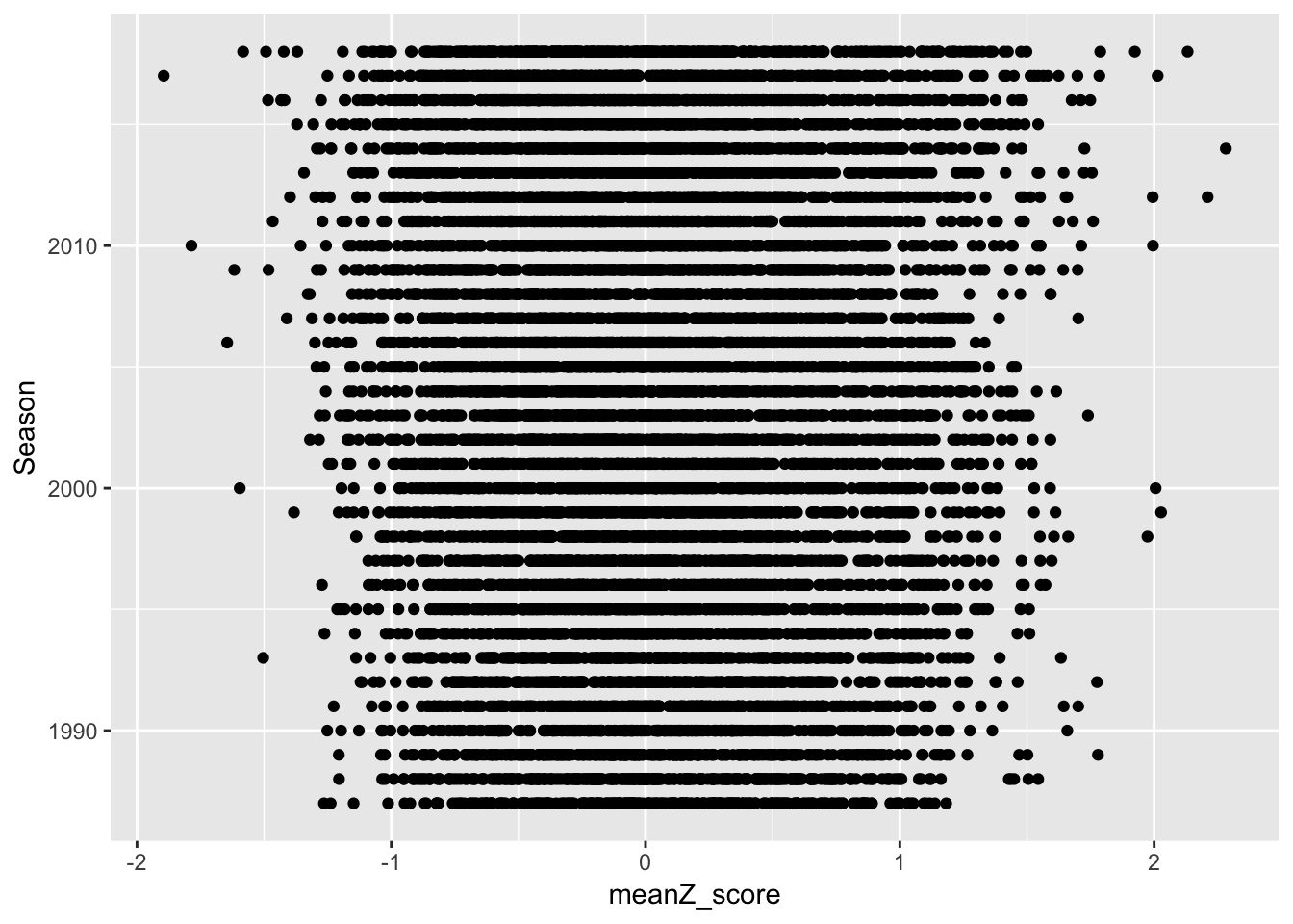
Then you probably would want to label our top 10 list so lets do that.
df%>%
  filter(Season>1986)%>%
  group_by(Season, ID)%>%
  mutate(countgames=n())%>%
  group_by(Season)%>%
  mutate(Z_score=(AF-mean(AF))/sd(AF))%>%
  group_by(Season, ID, First.name, Surname)%>%
filter(countgames>10)%>%
  summarise(meanZ_score=mean(Z_score))%>%
  ggplot(aes(x=meanZ_score, y=Season))+
  geom_point()+
  geom_text(aes(label=ifelse(meanZ_score>1.9, as.character(Surname),"")), vjust=2, size=2, colour="blue")+
  ggtitle("AFL Fantasy Z-Score by Season")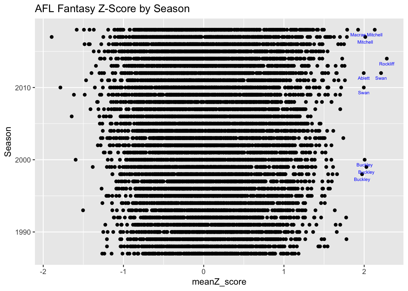
So what we can see here is that Nathan Buckley in his day, had some of the best fantasy seasons of AFL that we have statistics for. In fact, he has 3 out of the top 10 all time fantasy seasons.
It’s just a shame that fantasy wasn’t around back when he was around.
What about top 10 finishes?
df%>%
  filter(Season>1986)%>%
  group_by(Season, ID)%>%
  mutate(countgames=n())%>%
  group_by(Season)%>%
  mutate(Z_score=(AF-mean(AF))/sd(AF))%>%
  group_by(Season, ID, First.name, Surname)%>%
filter(countgames>10 & AF>30)%>%
  summarise(meanZ_score=mean(Z_score))%>%
   group_by(Season) %>%
  arrange(desc(meanZ_score))%>%
  mutate(id = row_number())%>%
  filter(id<11)%>%
  group_by(ID, First.name, Surname)%>%summarise(top10=n())%>%
  arrange(desc(top10))
## # A tibble: 150 x 4
## # Groups: ID, First.name [150]
## ID First.name Surname top10
## <dbl> <chr> <chr> <int>
## 1 217 Nathan Buckley 11
## 2 1105 Gary Ablett 9
## 3 1460 Dane Swan 9
## 4 766 Wayne Carey 7
## 5 990 Tony Lockett 7
## 6 157 Barry Mitchell 6
## 7 927 Stewart Loewe 6
## 8 4182 Scott Pendlebury 6
## 9 142 Greg Williams 5
## 10 312 James Hird 5
## # … with 140 more rowsYes there you have it, not only does he have some of the best seasons of fantasy relative to the other players in his season group. But he also has the most number of top10 fantasy finishes in “possible” fantasy history( if we started when tackles first started getting recorded).