Hello and welcome to my new and improved blog. I have moved all my work from wordpress to github. This was done for a few reasons.
- Goal is to have reproducible work that readers can go away and play with themselves
- To get feedback on better ways of communication of how to use R and to get better at it myself.
- So that more people can get their hands on AFL data and do analysis they themselves find interesting.
So this week in AFL we have a couple of big milestones coming up. That of Scott Pendlebury and Gary Ablett. Usually with milestones and more so with big ones its always nice to do a player comparision. The following won’t be the most efficient way to do things (its not meant to be) but what it will hopefully show you is enough that if you were to have a go the steps to making it more efficient aren’t too far.
So the aim of this blog post is to
- Use some of the earlier leanings from other posts on how to scrape data using R
- Scrape player data using R
- Use some basic tidyverse to see some possibility interesting cuts of game data (of course hopefully from this you can cut data yourself to answer your questions).
The set up
We will be using R, so hopefully you already have the necessary packages installed, if not please see my earlier post on installing the right packages in R and setting yourself up with R Studio.
library(stringr)
library(XML)
library(rvest)
library(tidyr)
library(dplyr)
library(ggplot2)
What data are we after?
The data we want to get is the player data for every game that Scott Pendlebury and Gary Ablett have played in As a rule of thumb, when getting all the players data, a better way going forward might just to be to get all the data for all games for the time period since their respective debuts so we can not only compare Scott to Gary, but them to their peers. One of my favourite sites along with afltables is footywire
In this reproducible example I will be scraping game data from footywire.
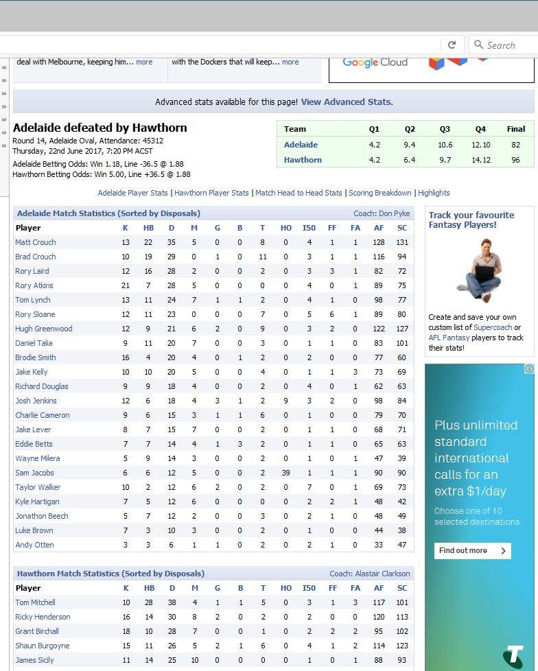
Looking at the image above we would want to not only get that game but all games from this year and last and the year before that etc.
Assuming we have the packages loaded, lets see how we can get the data!
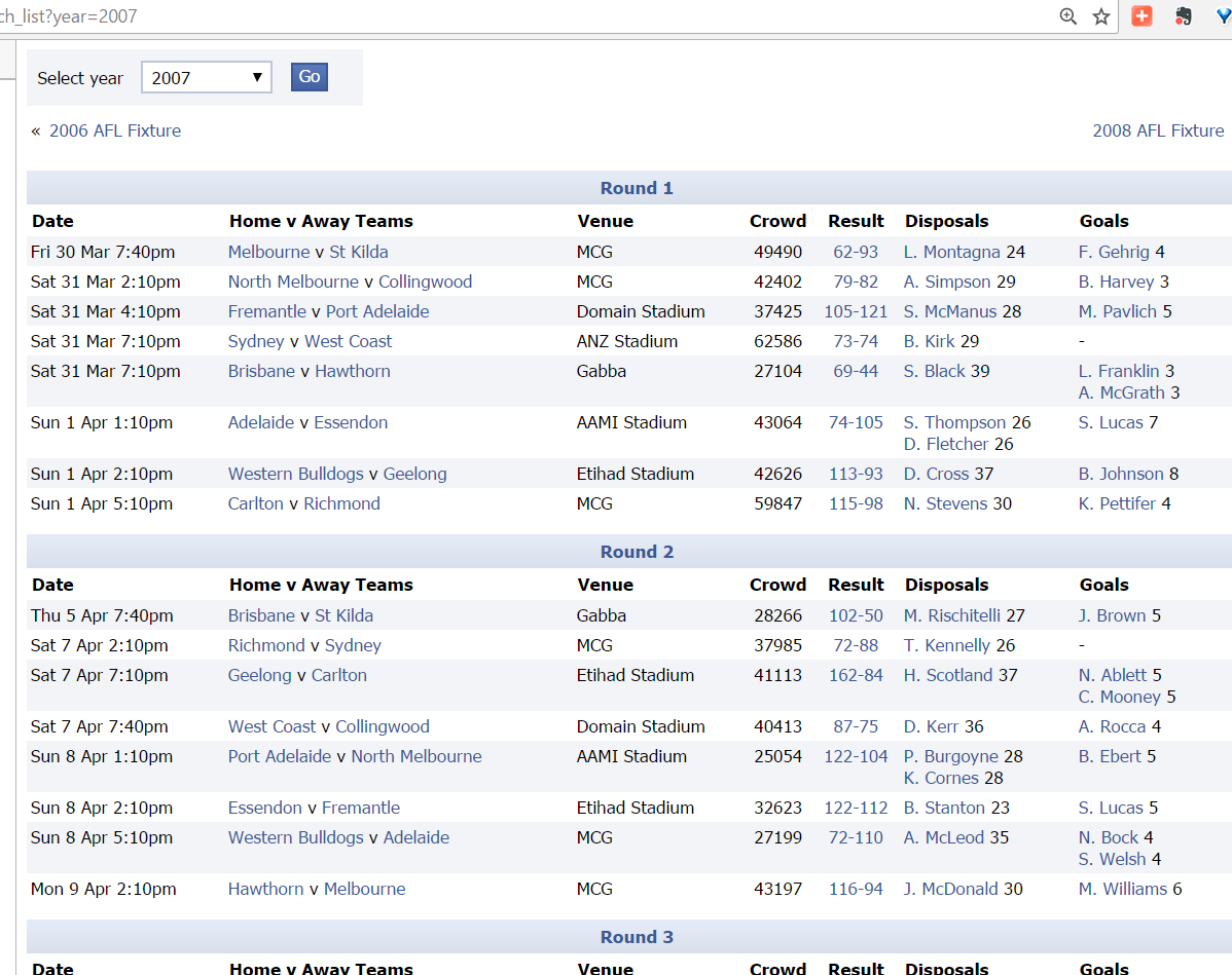
Screenshot of footywire site
 main.page<-read_html(x="http://www.footywire.com/afl/footy/ft_match_list?year=2007")
main.page
## {xml_document}
## <html>
## [1] <head>\n<meta http-equiv="Content-Type" content="text/html; charset= ...
## [2] <body onload="pushContent('Fixture', '2007');showMemberStatusWithUrl ...#just like the previous post, this will read all the html into RIf we were to manually do it, what we would do is we would click on each of the scores to go to the games. For example if we clicked on 62-93 it would take us to the page that contains the data from the Melbourne V St Kilda game Round 1 2007.
Now that sounds a bit tedius, so what we want to do at a high level is write some R code that allows us to click through on all the games for the year, go to the page and download the player statistics.
Step 1 Get all relevant URLS
To do that we need the script below.
urls<-main.page %>% ###get main page then we get links from main page
  html_nodes(".data:nth-child(5) a")%>%
  html_attr("href") #extract the urls

head(urls)
## [1] "ft_match_statistics?mid=2911" "ft_match_statistics?mid=2912"
## [3] "ft_match_statistics?mid=2913" "ft_match_statistics?mid=2915"
## [5] "ft_match_statistics?mid=2914" "ft_match_statistics?mid=2916"Now that we have done that we have all the URLS!
The part that must be looking very weird is the
 html_nodes(".data:nth-child(5) a")%>%
  html_attr("href") #extract the urls
So let me explain how I got that, another way to think about html_nodes is that its basically a way to get all the elements I want. Think about that in terms of, instead of clicking all the scores one by one to open a new page I just want them all at once.
So we use this chrome extension called selector gadget Once installed it will appear in your chrome like below.

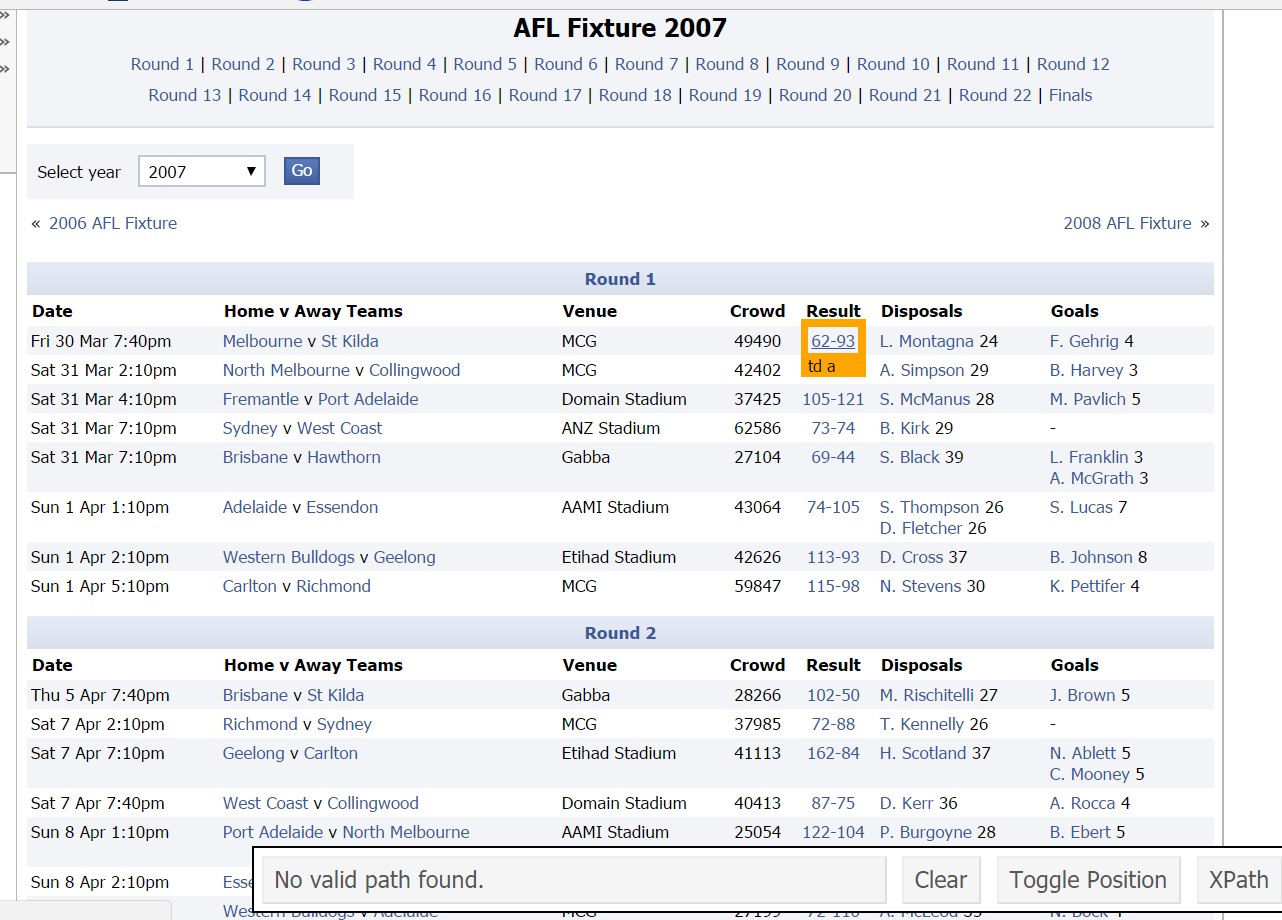
Selector Gadget
Looking at it, if you hover your mouse over the score from the Melbourne, Saints game in round 1 what do you get? Click on the score from the game and you will see this.
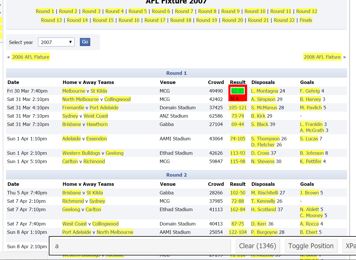
Selector Gadget
Now you can see that its highlighted what we want (all the scores) but it has also highlighted a lot of things we don’t want like the leading disposal winners, leading goal kickers the teams etc.
So our next click will be on something we don’t want say a leading possession getter like L.Montagna
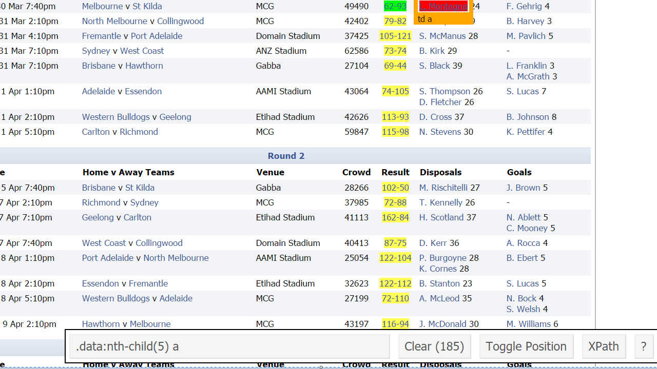
Selector Gadget
There we go that is how we got the “.data:nth-child(5) a” not that hard right?
Now what about the href?
That looks complex but let me show you how to get it!
Right click on the score of the Melbourne, St kilda game and you will get something like below, click on inspect
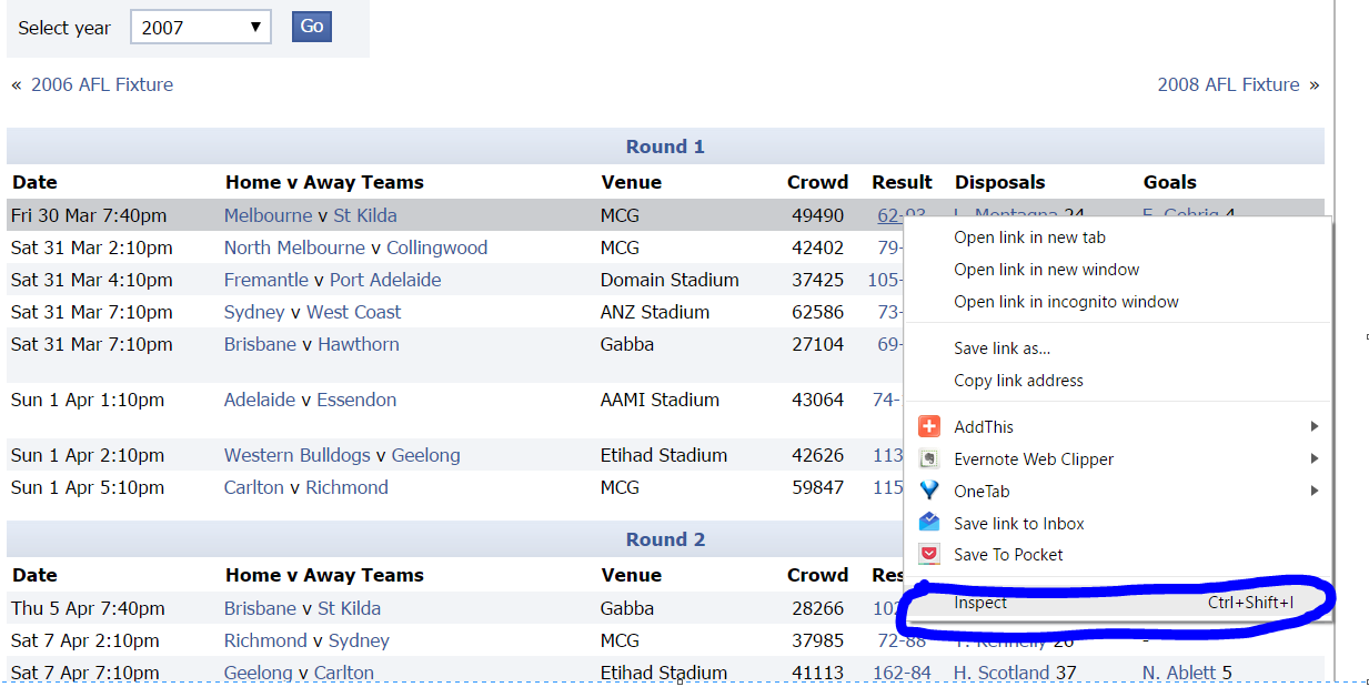
Selector Gadget
It should take you to a screen like

Selector Gadget
What do you notice about what is highlighted, we have the href which is a way to select all attributes that start with the string and if we look at the string, its leads us to the data in the Melbourne, St Kilda game!!
Step Two Another example - Lets get the scores!
OK so what we now have is the URLS to all the pages! Now lets get all the scores (match scores) that are related to the URLS we have just scraped
scores<-main.page%>%
    html_nodes(".data:nth-child(5) a")%>%
    html_text() ## gets us the scores
head(scores)
## [1] "62-93" "79-82" "105-121" "73-74" "69-44" "74-105"So now we have all the links, hopefully doing the score example you have gotten a better idea about how to pull different bits of data from the web!
Now lets align the score data with the urls, this might not make a lot of sense now but it will hopefully later on.
matchstats<-data.frame(scores=scores,urls=urls,stringsAsFactors = FALSE)
 head(matchstats)
## scores urls
## 1 62-93 ft_match_statistics?mid=2911
## 2 79-82 ft_match_statistics?mid=2912
## 3 105-121 ft_match_statistics?mid=2913
## 4 73-74 ft_match_statistics?mid=2915
## 5 69-44 ft_match_statistics?mid=2914
## 6 74-105 ft_match_statistics?mid=2916Evaluating that we get something like above.
Which if we look closely is the score from the game (link) next to the URL of the game!
What we notice about the url is that the only thing that changes is the number at the end, so lets separate this out. (This makes things easier down the track)
x1<- matchstats%>%
      separate(urls,c("urls","ID"),sep="=")
head(x1)
## scores urls ID
## 1 62-93 ft_match_statistics?mid 2911
## 2 79-82 ft_match_statistics?mid 2912
## 3 105-121 ft_match_statistics?mid 2913
## 4 73-74 ft_match_statistics?mid 2915
## 5 69-44 ft_match_statistics?mid 2914
## 6 74-105 ft_match_statistics?mid 2916Step Three Get the Data
default.url <-  "http://www.footywire.com/afl/footy/ft_match_statistics?mid="
    basic  <-  data.frame()
    for (i in x1$ID) {
      i=i
    print(i) ##prints data as it runs so we don't wait till end
    sel.url      <-  paste(default.url, i, sep="") ##paste forms the url, try a test case when i=2999 and run and see what happens
    htmlcode     <- readLines(sel.url) ###in the same test case type htmlcode hit enter
    export.table <- readHTMLTable(htmlcode) ##like the example before, gets all the tables
    top.table    <- as.data.frame(export.table[13]) ##looking at tables, 13 is the top one
    bot.table    <- as.data.frame(export.table[17]) ## 17 is the bottom table
    ind.table    <- rbind(top.table, bot.table) ##rbind, binds the top table to the bottom table
    ind.table$MatchId <- rep(i, nrow(ind.table)) ##this is adding a match ID which is the unique end of the url
    print(summary(ind.table))
    basic  <- rbind(basic, ind.table)
    }
basic
 default.url <-  "http://www.footywire.com/afl/footy/ft_match_statistics?mid="
    basic  <-  data.frame()
    # for (i in x1$ID) {
      i=2999
      print(i) ##prints data as it runs so we don't wait till end
      sel.url      <-  paste(default.url, i, sep="") ##paste forms the url, try a test case when i=2999 and run and see what happens
      sel.url
      htmlcode     <- readLines(sel.url) ###in the same test case type htmlcode hit enter
      htmlcode
      export.table <- readHTMLTable(htmlcode) ##like the example before, gets all the tables
      export.table
      top.table    <- as.data.frame(export.table[13]) ##looking at tables, 13 is the top one
      top.table
      bot.table    <- as.data.frame(export.table[17]) ## 17 is the bottom table
      bot.table
      ind.table    <- rbind(top.table, bot.table) ##rbind, binds the top table to the bottom table
      ind.table
      ind.table$MatchId <- rep(i, nrow(ind.table)) ##this is adding a match ID which is the unique end of the url
      ind.table
      print(summary(ind.table))
      basic  <- rbind(basic, ind.table)
      basic
      # }
basic
In this case scores which just happened to be the link which we click on to go to the relevant game. We couldn’t use something like clicking on any of the teams, because this would take us through to the team page. For example if we clicked on Melbourne we would go here.
But we can see its relevance from the way our table looks like. What we would also want is not only the player statistics, but we would want maybe a column for their team that they are in?
We can use the following to get the team names and then relate them to the urls and combine them with the scores.
    main.page<-read_html(x="http://www.footywire.com/afl/footy/ft_match_list?year=2007")

  urls<-main.page %>% ###get main page then we get links from main page
    html_nodes(".data:nth-child(5) a")%>%
    html_attr("href") #extract the urls
  head(urls)
## [1] "ft_match_statistics?mid=2911" "ft_match_statistics?mid=2912"
## [3] "ft_match_statistics?mid=2913" "ft_match_statistics?mid=2915"
## [5] "ft_match_statistics?mid=2914" "ft_match_statistics?mid=2916" scores<-main.page%>%
html_nodes(".data:nth-child(5) a")%>%
html_text()
head(scores)## [1] "62-93" "79-82" "105-121" "73-74" "69-44" "74-105" team.names<-main.page%>%
html_nodes(".data:nth-child(2)")%>%
html_text()
head(team.names)## [1] "\nMelbourne\nv \nSt Kilda\n"
## [2] "\nNorth Melbourne\nv \nCollingwood\n"
## [3] "\nFremantle\nv \nPort Adelaide\n"
## [4] "\nSydney\nv \nWest Coast\n"
## [5] "\nBrisbane\nv \nHawthorn\n"
## [6] "\nAdelaide\nv \nEssendon\n" matchstats<-data.frame(team.names=team.names,scores=scores,urls=urls,stringsAsFactors = FALSE)
head(matchstats)## team.names scores
## 1 \nMelbourne\nv \nSt Kilda\n 62-93
## 2 \nNorth Melbourne\nv \nCollingwood\n 79-82
## 3 \nFremantle\nv \nPort Adelaide\n 105-121
## 4 \nSydney\nv \nWest Coast\n 73-74
## 5 \nBrisbane\nv \nHawthorn\n 69-44
## 6 \nAdelaide\nv \nEssendon\n 74-105
## urls
## 1 ft_match_statistics?mid=2911
## 2 ft_match_statistics?mid=2912
## 3 ft_match_statistics?mid=2913
## 4 ft_match_statistics?mid=2915
## 5 ft_match_statistics?mid=2914
## 6 ft_match_statistics?mid=2916Ideally we would want columns for the home team, away team, home score and away score.
We can do that with the following script:
main.page<-read_html(x="http://www.footywire.com/afl/footy/ft_match_list?year=2007")
urls<-main.page %>% ###get main page then we get links from main page
html_nodes(".data:nth-child(5) a")%>%
html_attr("href") #extract the urls
scores<-main.page%>%
html_nodes(".data:nth-child(5) a")%>%
html_text()
team.names<-main.page%>%
html_nodes(".data:nth-child(2)")%>%
html_text()
  matchstats<-data.frame(team.names=team.names,scores=scores,urls=urls,stringsAsFactors = FALSE)
  head(matchstats)
## team.names scores
## 1 \nMelbourne\nv \nSt Kilda\n 62-93
## 2 \nNorth Melbourne\nv \nCollingwood\n 79-82
## 3 \nFremantle\nv \nPort Adelaide\n 105-121
## 4 \nSydney\nv \nWest Coast\n 73-74
## 5 \nBrisbane\nv \nHawthorn\n 69-44
## 6 \nAdelaide\nv \nEssendon\n 74-105
## urls
## 1 ft_match_statistics?mid=2911
## 2 ft_match_statistics?mid=2912
## 3 ft_match_statistics?mid=2913
## 4 ft_match_statistics?mid=2915
## 5 ft_match_statistics?mid=2914
## 6 ft_match_statistics?mid=2916x1<- matchstats%>%
separate(urls,c("urls","ID"),sep="=")
# x1 lets you see what you have just done
x2<-x1%>%separate(team.names,c("Home","Away"),sep="\nv")
# View(x2) another way to see what you have done
x3<-x2%>%separate(scores,c("home.score","away.score"),sep="-")
head(x3) ##looking at our final ID set## Home Away home.score away.score
## 1 \nMelbourne \nSt Kilda\n 62 93
## 2 \nNorth Melbourne \nCollingwood\n 79 82
## 3 \nFremantle \nPort Adelaide\n 105 121
## 4 \nSydney \nWest Coast\n 73 74
## 5 \nBrisbane \nHawthorn\n 69 44
## 6 \nAdelaide \nEssendon\n 74 105
## urls ID
## 1 ft_match_statistics?mid 2911
## 2 ft_match_statistics?mid 2912
## 3 ft_match_statistics?mid 2913
## 4 ft_match_statistics?mid 2915
## 5 ft_match_statistics?mid 2914
## 6 ft_match_statistics?mid 2916Of course you can work through the page yourself and add in items like the venue or the date, maybe you want the leading possession winner for the game etc.
Hopefully after all that you end up with something like below:
View(x3)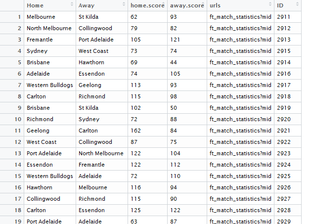
R output
In x3, we have a column called ID. In our basic dataset (the scraped player data we scraped earlier) we have an ID column called match ID. This is important because it means we can match the home team, away team and scores column to the players.
Why would you want to do that, maybe you want to see how a player performs against interstate teams only, so you need to have a record of not only the players in game statistics but the opposition. You might want to keep the scores because you have a feeling about players that just step up in close games. So you need the opposition and the playing teams scores.
So lets get started, our first step is we need to add a column for the top.table representing the home.team, the bot.table representing the away team. To do that we just add in 2 lines from what we did earlier and run the following.
default.url <-  "http://www.footywire.com/afl/footy/ft_match_statistics?mid="
basic  <-  data.frame()
for (i in x3$ID) {

  i=i #matchID

  print(i) ##prints data as it runs so we don't wait till end
  sel.url      <-  paste(default.url, i, sep="") ##paste forms the url, try a test case when i=2999 and run and see what happens
  # sel.url
  htmlcode     <- readLines(sel.url) ###in the same test case type htmlcode hit enter
  # htmlcode
  export.table <- readHTMLTable(htmlcode) ##like the example before, gets all the tables
  # export.table
  top.table    <- as.data.frame(export.table[13]) ##looking at tables, 13 is the top one
  top.table

  top.table$team <- "home.team"

  bot.table    <- as.data.frame(export.table[17]) ## 17 is the bottom table
  bot.table$team<-"away.team"
  ind.table    <- rbind(top.table, bot.table) ##rbind, binds the top table to the bottom table
  ind.table$MatchId <- rep(i, nrow(ind.table)) ##this is adding a match ID which is the unique end of the url
  print(summary(ind.table))
  basic  <- rbind(basic, ind.table)
  basic

}

View(basic)
If we do that we get something lovely like below
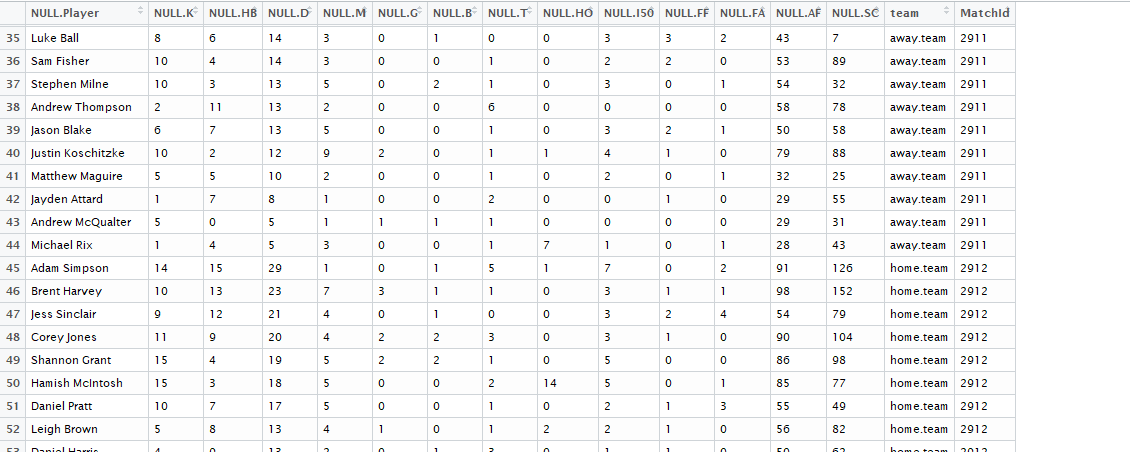
R output
Now lets just add in who the home team was, the away team was and the scores.
Merging the datasets
So this might seem a little bit tricky, but you will need to understand some new terms. I think a great source of information is stat545 website.
From here it looks as though a left join starting with basic should work.
dim(basic)
##we do dim because we want to know how many
#rows(observations) our dataset has
b<-left_join(basic,x3, by =c("MatchId"="ID"))
View(b)
dim(b)
If all runs smoothly we should end up with some output like below

R output
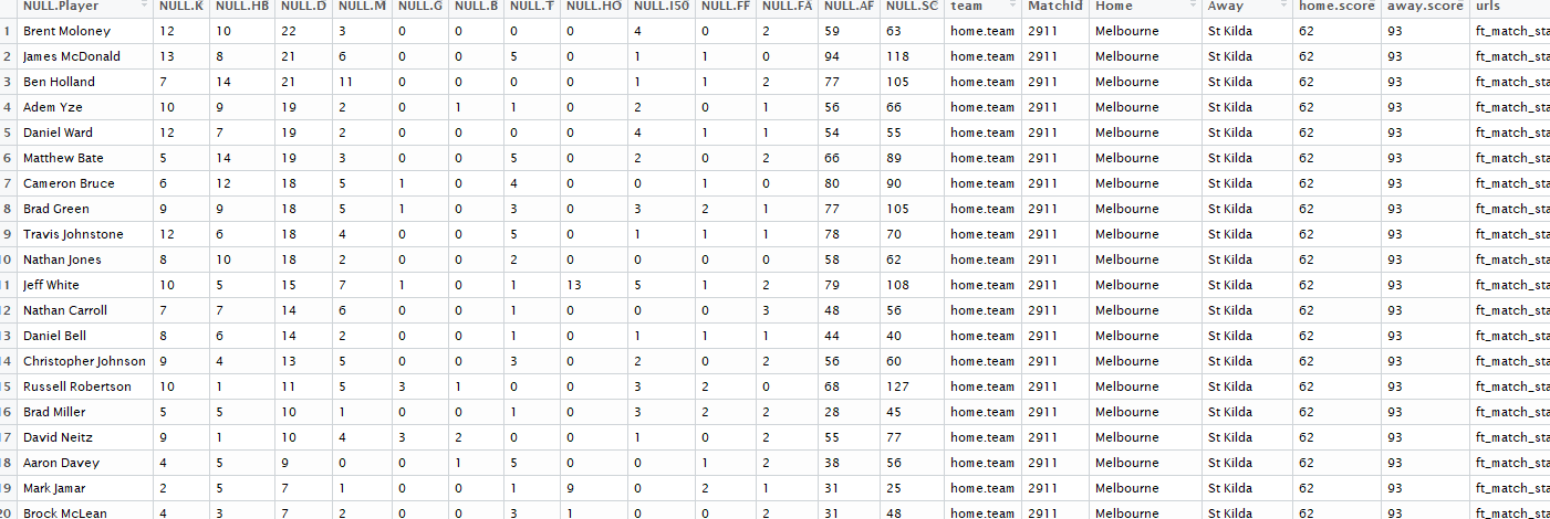
R output
We can see we have maintained our 8140 rows but we have added an additional 5 columns to our dataset and we have called it b.
So if you have been able to follow those instructions, the end output should be a completed dataset from 2007 that contains all of the player data in game from footywire. Hopefully you can now go away and get other years data!
Exploring the newly scraped data
So now you have got to the fun stuff, exploratory data analysis.
You want to explore your data before you go and do any modelling. Exploring your data has many benefits including but not limited too:
- Helping generate questions about your data
- Helping you identify trends
- Helping you understand variance of your variables
- Helping you spot anything weird about your data (missing values, incorrectly entered data, data that doesn’t make domain sense)
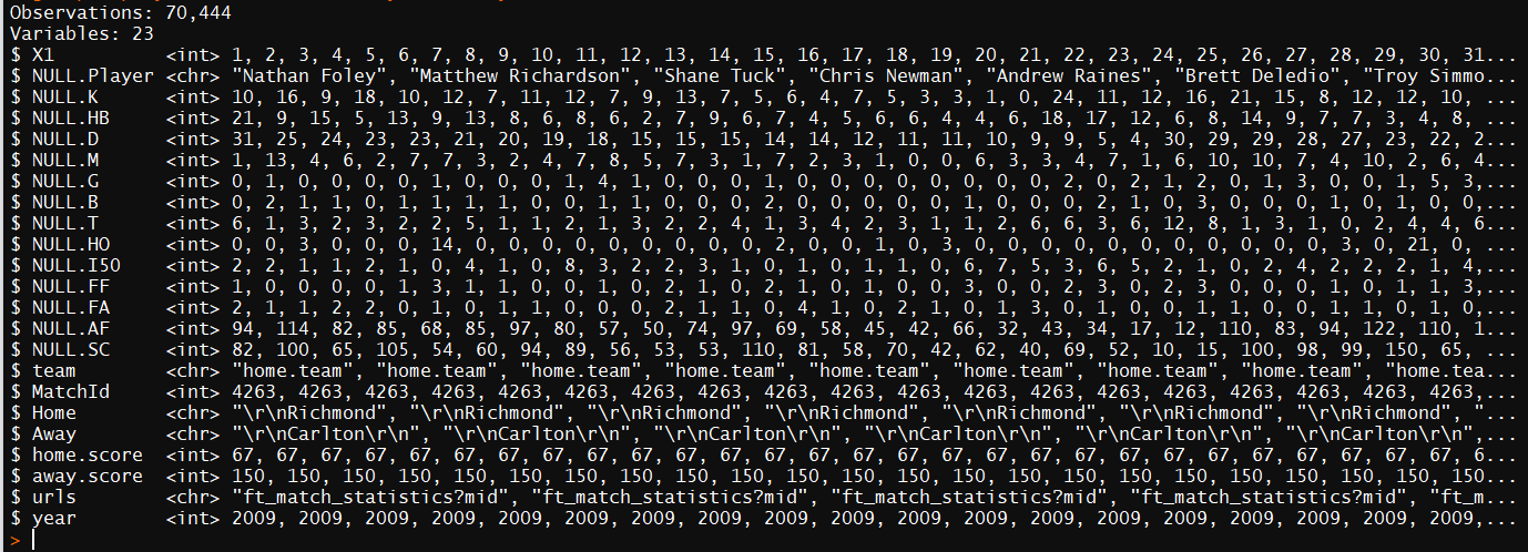
Hopefully you have gotten all the AFL data you want now, for this exploration I will be using the player data from 2009 to 2016. The reason I have chosen 2009 is because its Garys first Brownlow and the year Pendlebury first topped the Brownlow count for Collingwood.
library(dplyr)
library(ggplot2)
playerdata<- read_csv("C:/Users/put rest of the path to the file here/playerdata2009_20016.csv")
str(playerdata) ##one way to view your data
glimpse(playerdata) ##another way to view your data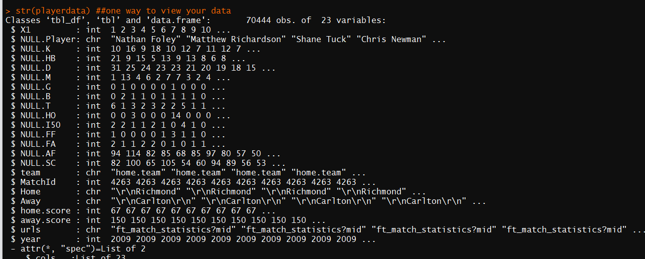
We want to understand our data, or at the very least get to know it better. As we get to know the data better we can start to drill down on the more interesting aspects of the data.
So if our goal is to get to know our data better one of the best ways is to look at the data visually. So lets plot some nice graphs.
Remember our goal at the start of this post (I know its long) was to explore Gary Ablett vs Scott Pendlebury
We will do this in the following order
- Filter out Gary and Scott
- plot their SC scores (because who hasn’t had them in their teams over the years)
post<-c("Scott Pendlebury","Gary Jnr Ablett") ##create a list of the players
##we want to filter out

data<-filter(playerdata,NULL.Player %in% post) ##filter out the players!

View(data)##view the data always!
R output
So now we have the dataset data that contains the gameday statistics for Gary Ablett and Scott Pendlebury, lets think of something interesting to see. From a personal standpoint, love SC and DT so lets look at their distribution of scores for Supercoach.
ggplot(data,aes(x=NULL.SC))+geom_density()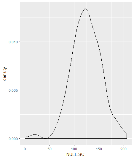
Denisty of Supercoach scores of Ablett and Pendlebury
That’s pretty interesting, but what if we looked at the densities of Ablett and Pendlebury on the same graph?
ggplot(data,aes(x=NULL.SC,colour=NULL.Player))+geom_density()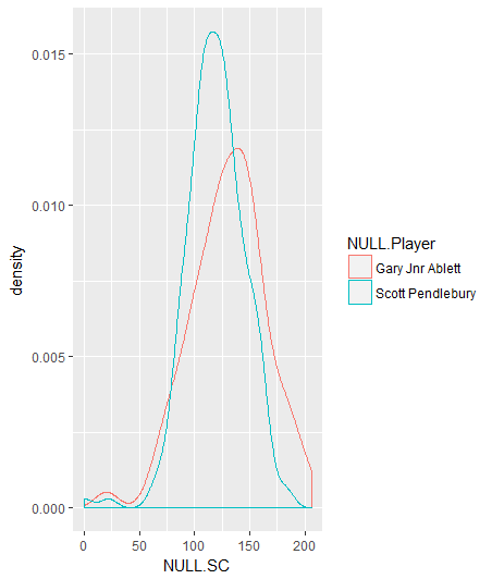
Denisty of Supercoach scores of Ablett and Pendlebury
What can we tell from that graph?
What about this graph instead?
ggplot(data,aes(x=NULL.Player,y=NULL.SC))+geom_boxplot()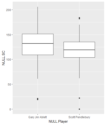
Boxplot of Supercoach scores of Ablett and Pendlebury
