Recently you might have seen an interesting ABC piece on Dustin Martin
In it it features some graphs built using data that has just recently become available in fitzRoy thanks to fryziggg who has kindly made it available for fans of afl statistics everywhere.
So what are the new things, and why is it cool. Well previously fitzRoy provided access to two pretty cool websites in afltables and footywire if you are a fan of AFL statistics you might already know the differences, but basically footywire had a few more game statistics than afltables but afltables provided data all the way back to the first game in 1897 while footywire did not.
Now more of you might be thinking oh but the AFL website itself has some more data available, but its just a pain to use. Its UI is pretty horrid, so its a little off putting having to manually copy and paste data into spreadsheets or its too much of a hurdle to go and learn how to scrape a website using R or python. But thankfully fryzigg has heard your frustrations and come along and help us make it more accessible for all.
So you might have read the Dustin Martin article and thought oh that’s cool but maybe I want to highlight some different players? While you can hover your mouse over the visualisation to label other players, that might not help you if you have no idea where your player of interest sits!
So How would you go about it and what are some things I think might be cool to explore a little differently.
In saying that, I want to make 3 changes to the graphs.
1 - I want the players I am interested in to to stand out more visually
2 - I want to be able to highlight players I am interested in
3 - I want to add a Season element to the plots, that is I want to be able to compare 2017 Dusty to 2016 Dusty and so on.
Lets first download the latest development version from github and create a Season column using lubridate::year
# devtools::install_github("jimmyday12/fitzRoy")
library(fitzRoy)
library(tidyverse)
## ── Attaching packages ─────────────────────────────────────────────────────────── tidyverse 1.3.0 ──## ✓ ggplot2 3.3.0 ✓ purrr 0.3.4
## ✓ tibble 3.0.1 ✓ dplyr 1.0.0
## ✓ tidyr 1.1.0 ✓ stringr 1.4.0
## ✓ readr 1.3.1 ✓ forcats 0.5.0## ── Conflicts ────────────────────────────────────────────────────────────── tidyverse_conflicts() ──
## x dplyr::filter() masks stats::filter()
## x dplyr::lag() masks stats::lag()df<-fitzRoy::get_fryzigg_stats(start=1897, end=2020)## Returning cached data from 1897 to 2020
## This may take some time.names(df)## [1] "venue_name" "match_id"
## [3] "match_home_team" "match_away_team"
## [5] "match_date" "match_local_time"
## [7] "match_attendance" "match_round"
## [9] "match_home_team_goals" "match_home_team_behinds"
## [11] "match_home_team_score" "match_away_team_goals"
## [13] "match_away_team_behinds" "match_away_team_score"
## [15] "match_margin" "match_winner"
## [17] "match_weather_temp_c" "match_weather_type"
## [19] "player_id" "player_first_name"
## [21] "player_last_name" "player_height_cm"
## [23] "player_weight_kg" "player_is_retired"
## [25] "player_team" "guernsey_number"
## [27] "kicks" "marks"
## [29] "handballs" "disposals"
## [31] "effective_disposals" "disposal_efficiency_percentage"
## [33] "goals" "behinds"
## [35] "hitouts" "tackles"
## [37] "rebounds" "inside_fifties"
## [39] "clearances" "clangers"
## [41] "free_kicks_for" "free_kicks_against"
## [43] "brownlow_votes" "contested_possessions"
## [45] "uncontested_possessions" "contested_marks"
## [47] "marks_inside_fifty" "one_percenters"
## [49] "bounces" "goal_assists"
## [51] "time_on_ground_percentage" "afl_fantasy_score"
## [53] "supercoach_score" "centre_clearances"
## [55] "stoppage_clearances" "score_involvements"
## [57] "metres_gained" "turnovers"
## [59] "intercepts" "tackles_inside_fifty"
## [61] "contest_def_losses" "contest_def_one_on_ones"
## [63] "contest_off_one_on_ones" "contest_off_wins"
## [65] "def_half_pressure_acts" "effective_kicks"
## [67] "f50_ground_ball_gets" "ground_ball_gets"
## [69] "hitouts_to_advantage" "hitout_win_percentage"
## [71] "intercept_marks" "marks_on_lead"
## [73] "pressure_acts" "rating_points"
## [75] "ruck_contests" "score_launches"
## [77] "shots_at_goal" "spoils"
## [79] "subbed" "player_position"df$Season<-lubridate::year(df$match_date)Next part, is we want to create the data to plot, to do this we want reproduce the plot that has the average number of centre clearances won on the x axis and the average number of stoppage clearances won on the y axis. The other things we want to do is filter our data by number of games played in season, I am going to set this number to 15
We will do this and call that dataframe p
p<-df%>%
group_by(Season,player_id, player_first_name, player_last_name)%>%
  summarise(mean_centre_clearances=mean(centre_clearances, na.rm=TRUE), mean_clear=mean(stoppage_clearances,na.rm=TRUE),no_games=n())%>%
  filter(Season>2011)%>%
  filter(no_games>14)
## `summarise()` regrouping output by 'Season', 'player_id', 'player_first_name' (override with `.groups` argument)Now if we were to take p and use facet_wrap(~Season) we get a heap of black dots geom_point().
p%>%
   ggplot(aes(x=mean_clear, y=mean_centre_clearances,label=paste(player_first_name, player_last_name)))+geom_point() +facet_wrap(~Season)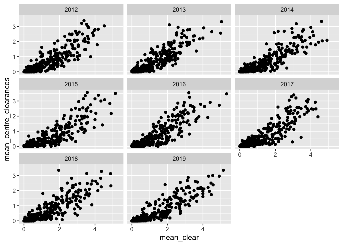
Now we want to create a dataset with our players of interest one way to do this is using their unique player IDS which has been kindly provided by Fryzigg. These align to the official champion data IDS where possible, which is really cool, if you are so lucky it might mean you can append all the secret sauce AFL statistics that are withheld from fans to your insights.
p_subset<-p%>%
  filter(player_id %in% c(11706, # Patrick Dangerfield
                          11801, # Dustin Martin
                          11844, # Nat Fyfe
                          12269, # Patrick Cripps
                          12061, # Lachie Neale
                          11813, # Luke Shuey
                          12058, # Adam Treloar
                          12223, # Brodie Grundie
                          11506, # Scott Pendlebury
                          12605, # Tim Kelly
                          12277 , # Marcus Bontempelli
                          11170   #Gary Ablett Jr
                          ))

p_subset_dusty<-p%>%
  filter(player_id %in% c(11801))
So how do we make our players of interest pop out a bit more on the graph?
Well lets plot all the relevant players in our dataset in a lighter colour say grey and over that, we plot our players of interest in a darker colour say black.
p%>%
   ggplot(aes(x=mean_clear, y=mean_centre_clearances,label=paste(player_first_name, player_last_name)))+
  geom_point(colour="grey", alpha=0.4)+ # all the data
   geom_point(data=p_subset, colour="black")+ # subset of players of interest
  geom_text(data=p_subset, size=2)+
facet_wrap(~Season)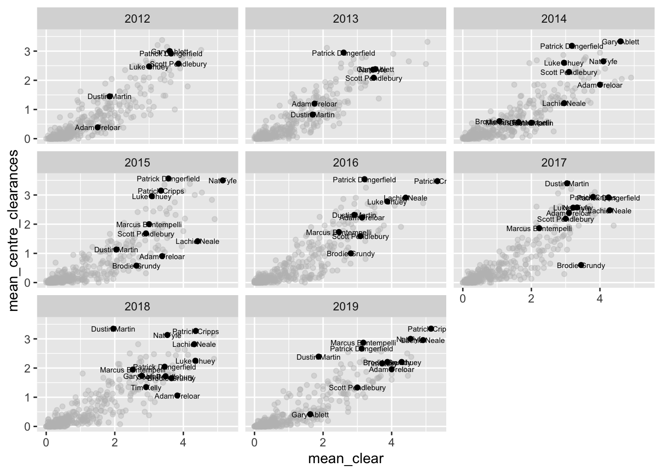
p%>%
   ggplot(aes(x=mean_clear, y=mean_centre_clearances,label=paste(player_first_name, player_last_name)))+
  geom_point(colour="grey", alpha=0.4)+ # all the data
   geom_point(data=p_subset_dusty, colour="black")+ # subset of players of interest
  geom_text(data=p_subset_dusty, size=2)+
facet_wrap(~Season)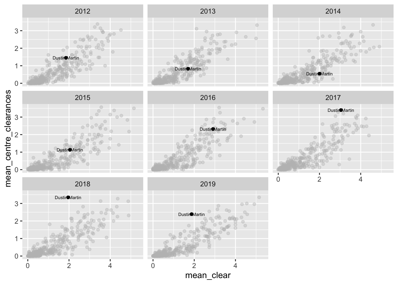
So I think that is a pretty handy template if you want to explore so what exactly can you explore?
names(df)## [1] "venue_name" "match_id"
## [3] "match_home_team" "match_away_team"
## [5] "match_date" "match_local_time"
## [7] "match_attendance" "match_round"
## [9] "match_home_team_goals" "match_home_team_behinds"
## [11] "match_home_team_score" "match_away_team_goals"
## [13] "match_away_team_behinds" "match_away_team_score"
## [15] "match_margin" "match_winner"
## [17] "match_weather_temp_c" "match_weather_type"
## [19] "player_id" "player_first_name"
## [21] "player_last_name" "player_height_cm"
## [23] "player_weight_kg" "player_is_retired"
## [25] "player_team" "guernsey_number"
## [27] "kicks" "marks"
## [29] "handballs" "disposals"
## [31] "effective_disposals" "disposal_efficiency_percentage"
## [33] "goals" "behinds"
## [35] "hitouts" "tackles"
## [37] "rebounds" "inside_fifties"
## [39] "clearances" "clangers"
## [41] "free_kicks_for" "free_kicks_against"
## [43] "brownlow_votes" "contested_possessions"
## [45] "uncontested_possessions" "contested_marks"
## [47] "marks_inside_fifty" "one_percenters"
## [49] "bounces" "goal_assists"
## [51] "time_on_ground_percentage" "afl_fantasy_score"
## [53] "supercoach_score" "centre_clearances"
## [55] "stoppage_clearances" "score_involvements"
## [57] "metres_gained" "turnovers"
## [59] "intercepts" "tackles_inside_fifty"
## [61] "contest_def_losses" "contest_def_one_on_ones"
## [63] "contest_off_one_on_ones" "contest_off_wins"
## [65] "def_half_pressure_acts" "effective_kicks"
## [67] "f50_ground_ball_gets" "ground_ball_gets"
## [69] "hitouts_to_advantage" "hitout_win_percentage"
## [71] "intercept_marks" "marks_on_lead"
## [73] "pressure_acts" "rating_points"
## [75] "ruck_contests" "score_launches"
## [77] "shots_at_goal" "spoils"
## [79] "subbed" "player_position"
## [81] "Season"So all this available in fitzRoy. Now that you know and hopefully have some script to one, what would you as a fan like to explore?