Using fitzRoy and the tidyverse
library(fitzRoy)
library(tidyverse)
## -- Attaching packages ----------------------- tidyverse 1.2.1 --## v ggplot2 2.2.1 v purrr 0.2.5
## v tibble 1.4.2 v dplyr 0.7.6
## v tidyr 0.8.1 v stringr 1.3.1
## v readr 1.1.1 v forcats 0.3.0## -- Conflicts -------------------------- tidyverse_conflicts() --
## x dplyr::filter() masks stats::filter()
## x dplyr::lag() masks stats::lag()So what we did before, was we created 3 variables from afltables about Tony Lockett. They were Year (afl season), GM (totals games played in afl season) and GL (total goals kicked in season).
These are summary statistics i.e. the year summaries (totals) of games played and goals kicked.
Something you might have noticed with fitzRoy is that the df is stored as game by game data and not season summaries.
So how do we create these summary statistics?
Step One - Get the dataframe with it all
Data is stored in different places in fitzRoy, df contains the data we are after at the moment
head(df)
options(max.print=20)
df<-fitzRoy::get_afltables_stats(start_date = "1897-01-01", end_date = Sys.Date())
## Returning data from 1897-01-01 to 2018-09-04## Downloading data##
## Finished downloading data. Processing XMLs## Warning: Unknown columns: `Substitute`## Finished getting afltables dataStep Two - Select the columns that you want select
df%>%
  select(First.name, Surname, Season, Goals)
## Adding missing grouping variables: `Round`, `Home.team`, `Away.team`## # A tibble: 619,992 x 7
## # Groups: Season, Round, Home.team, Away.team [15,398]
## Round Home.team Away.team First.name Surname Season Goals
## <chr> <chr> <chr> <chr> <chr> <dbl> <dbl>
## 1 1 Fitzroy Carlton Bill Ahern 1897 0
## 2 1 Fitzroy Carlton Jimmy Aitken 1897 0
## 3 1 Fitzroy Carlton Bob Armstrong 1897 0
## 4 1 Fitzroy Carlton Tom Blake 1897 0
## 5 1 Fitzroy Carlton Otto Buck 1897 0
## 6 1 Fitzroy Carlton Bob Cameron 1897 0
## 7 1 Fitzroy Carlton Bill Casey 1897 0
## 8 1 Fitzroy Carlton Arthur Cummins 1897 0
## 9 1 Fitzroy Carlton Henry Dunne 1897 0
## 10 1 Fitzroy Carlton Brook Hannah 1897 0
## # ... with 619,982 more rowsStep Three - Create the grouped data group_by
Now this might seem a bit weird, because on first look it would seem as though group_by doesn’t do anything.
df%>%
  select(First.name, Surname, Season, Goals)%>%
  group_by(Season)
## Adding missing grouping variables: `Round`, `Home.team`, `Away.team`## # A tibble: 619,992 x 7
## # Groups: Season [122]
## Round Home.team Away.team First.name Surname Season Goals
## <chr> <chr> <chr> <chr> <chr> <dbl> <dbl>
## 1 1 Fitzroy Carlton Bill Ahern 1897 0
## 2 1 Fitzroy Carlton Jimmy Aitken 1897 0
## 3 1 Fitzroy Carlton Bob Armstrong 1897 0
## 4 1 Fitzroy Carlton Tom Blake 1897 0
## 5 1 Fitzroy Carlton Otto Buck 1897 0
## 6 1 Fitzroy Carlton Bob Cameron 1897 0
## 7 1 Fitzroy Carlton Bill Casey 1897 0
## 8 1 Fitzroy Carlton Arthur Cummins 1897 0
## 9 1 Fitzroy Carlton Henry Dunne 1897 0
## 10 1 Fitzroy Carlton Brook Hannah 1897 0
## # ... with 619,982 more rowsIt doesn’t look like our dataset has changed, but if we look closely we have a new Groups: Season [121] and hopefully what you have noticed is that our dataset df has 121 unique values for Season. Which we can check below.
length(unique(df$Season))## [1] 122What this does is adds a grouping structure to our data, which means instead of operations acting element wise like they did earlier now operations can happen by group.
So why would you want to group data? Well lots of interesting things are done on a group_by basis. For example we might be interested in goal kicking trends by Season Or * by round * by Playing.For * by opponent * by wins and losses
We can also group_by more than one thing. For example what if we wanted by Season and Round
df%>%
  select(Season,Round, Goals, Behinds)%>%
  group_by(Season, Round)
## Adding missing grouping variables: `Home.team`, `Away.team`## # A tibble: 619,992 x 6
## # Groups: Season, Round [2,817]
## Home.team Away.team Season Round Goals Behinds
## <chr> <chr> <dbl> <chr> <dbl> <dbl>
## 1 Fitzroy Carlton 1897 1 0 0
## 2 Fitzroy Carlton 1897 1 0 0
## 3 Fitzroy Carlton 1897 1 0 0
## 4 Fitzroy Carlton 1897 1 0 0
## 5 Fitzroy Carlton 1897 1 0 0
## 6 Fitzroy Carlton 1897 1 0 0
## 7 Fitzroy Carlton 1897 1 0 0
## 8 Fitzroy Carlton 1897 1 0 0
## 9 Fitzroy Carlton 1897 1 0 0
## 10 Fitzroy Carlton 1897 1 0 0
## # ... with 619,982 more rowsWhat we can now see is that we have grouped by 2 variables (Season, Round) and have formed 769 groups. Groups: Season, Round [2,769]
Step Four - Take the grouped data and summarise it
So recall earlier we grouped our data by year so lets summarise it.
df%>%
  select(First.name, Surname, Season, Goals)%>%
  group_by(Season)%>%
  summarise(total_goals=sum(Goals))
## Adding missing grouping variables: `Round`, `Home.team`, `Away.team`## # A tibble: 122 x 2
## Season total_goals
## <dbl> <dbl>
## 1 1897 640
## 2 1898 721
## 3 1899 691
## 4 1900 750
## 5 1901 847
## 6 1902 878
## 7 1903 890
## 8 1904 949
## 9 1905 984
## 10 1906 1088
## # ... with 112 more rowsOk that doesn’t quite seem like what we were thinking we wanted the total_goals of Tony Lockett by season, but all we got was Season total goals.
Well duh! We only did a group_by by Season, we should have done it by Season, First.name, Surname should we have?
Lets check.
df%>%
  select(Season, First.name, Surname, Goals)%>%
  group_by(Season, First.name, Surname)%>%
  summarise(total_goals=sum(Goals))
## Adding missing grouping variables: `Round`, `Home.team`, `Away.team`## # A tibble: 53,330 x 4
## # Groups: Season, First.name [?]
## Season First.name Surname total_goals
## <dbl> <chr> <chr> <dbl>
## 1 1897 Alb Thomas 0
## 2 1897 Alby Patterson 0
## 3 1897 Alby Stamp 0
## 4 1897 Alby Tame 0
## 5 1897 Alec Sloan 0
## 6 1897 Alex Davidson 0
## 7 1897 Alex Murdoch 0
## 8 1897 Alf Bedford 0
## 9 1897 Alf Healing 0
## 10 1897 Alf Pontin 1
## # ... with 53,320 more rowsThis looks a lot better, only issue is that we don’t see Tony Lockett but we see all these other blokes like Alb Thomas, he didn’t kick 1,360 snags.
Step five - filter the data
df%>%
  select(Season, First.name, Surname, Goals)%>%
  group_by(Season, First.name, Surname)%>%
  summarise(total_goals=sum(Goals))%>%
  filter(First.name=="Tony" , Surname=="Lockett")
## Adding missing grouping variables: `Round`, `Home.team`, `Away.team`## # A tibble: 18 x 4
## # Groups: Season, First.name [18]
## Season First.name Surname total_goals
## <dbl> <chr> <chr> <dbl>
## 1 1983 Tony Lockett 19
## 2 1984 Tony Lockett 77
## 3 1985 Tony Lockett 79
## 4 1986 Tony Lockett 60
## 5 1987 Tony Lockett 117
## 6 1988 Tony Lockett 35
## 7 1989 Tony Lockett 78
## 8 1990 Tony Lockett 65
## 9 1991 Tony Lockett 127
## 10 1992 Tony Lockett 132
## 11 1993 Tony Lockett 53
## 12 1994 Tony Lockett 56
## 13 1995 Tony Lockett 110
## 14 1996 Tony Lockett 121
## 15 1997 Tony Lockett 37
## 16 1998 Tony Lockett 109
## 17 1999 Tony Lockett 82
## 18 2002 Tony Lockett 3Now I think I might know what you are thinking. “Weren’t we supposed to be plotting average goals by year?”
To do that all we have to do is change sum to mean and total_goals to average_goals (these names can be anything but its helpful if they are descriptive).
df%>%
  select(Season, First.name, Surname, Goals)%>%
  group_by(Season, First.name, Surname)%>%
  summarise(average_goals=mean(Goals))%>%
  filter(First.name=="Tony" , Surname=="Lockett")
## Adding missing grouping variables: `Round`, `Home.team`, `Away.team`## # A tibble: 18 x 4
## # Groups: Season, First.name [18]
## Season First.name Surname average_goals
## <dbl> <chr> <chr> <dbl>
## 1 1983 Tony Lockett 1.58
## 2 1984 Tony Lockett 3.85
## 3 1985 Tony Lockett 3.76
## 4 1986 Tony Lockett 3.33
## 5 1987 Tony Lockett 5.32
## 6 1988 Tony Lockett 4.38
## 7 1989 Tony Lockett 7.09
## 8 1990 Tony Lockett 5.42
## 9 1991 Tony Lockett 7.47
## 10 1992 Tony Lockett 6
## 11 1993 Tony Lockett 5.3
## 12 1994 Tony Lockett 5.6
## 13 1995 Tony Lockett 5.79
## 14 1996 Tony Lockett 5.5
## 15 1997 Tony Lockett 3.08
## 16 1998 Tony Lockett 4.74
## 17 1999 Tony Lockett 4.32
## 18 2002 Tony Lockett 1Step Six - ggplot our way to a glory
df%>%
  select(Season, First.name, Surname, Goals)%>%
  group_by(Season, First.name, Surname)%>%
  summarise(average_goals=mean(Goals))%>%
  filter(First.name=="Tony" , Surname=="Lockett")%>%
  ggplot(aes(x=Season, y=average_goals)) +
  geom_line(color="red") +
  ggtitle("Tony Lockets Average Goals Per Game by Season")
## Adding missing grouping variables: `Round`, `Home.team`, `Away.team`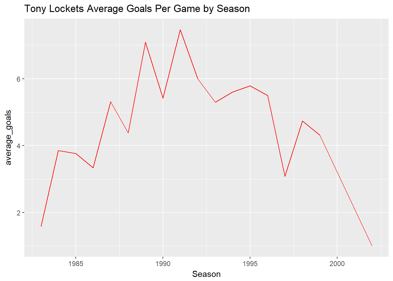
Step 7 - That’s cool but I want to compare players
To do this the obvious thing to do, is to just add a player you want to compare to the filter we do this with %in% c("Player1",("Player2"))
df%>%
  select(Season, First.name, Surname, Goals)%>%
  group_by(Season, First.name, Surname)%>%
  summarise(average_goals=mean(Goals))%>%
  filter(First.name %in% c("Tony", "Jason") , Surname %in% c("Lockett", "Dunstall"))%>%
  ggplot(aes(x=Season, y=average_goals)) +
  geom_line() +
  ggtitle("Average Goals Per Game by Season")
## Adding missing grouping variables: `Round`, `Home.team`, `Away.team`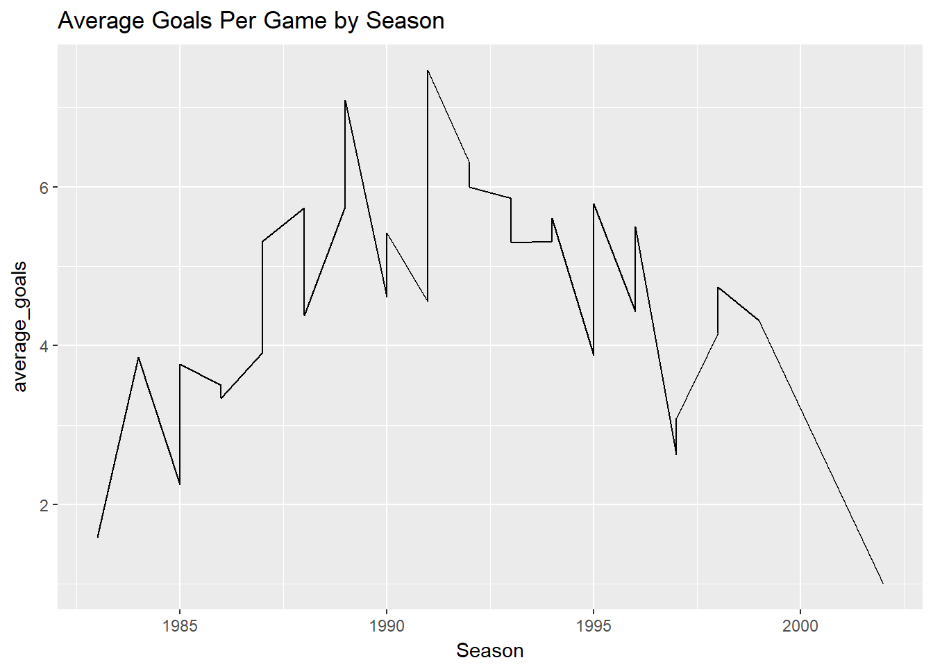
On first glance this doesn’t look like its done the right thing we wanted two lines one for Tony Lockett and one for Jason Dunstall.
Lets look a bit deeper at what we are doing
Look at the dataframe is it what we wanted?
df%>%
  select(Season, First.name, Surname, Goals)%>%
  group_by(Season, First.name, Surname)%>%
  summarise(average_goals=mean(Goals))%>%
  filter(First.name %in% c("Tony", "Jason") , Surname %in% c("Lockett", "Dunstall"))
## Adding missing grouping variables: `Round`, `Home.team`, `Away.team`## # A tibble: 32 x 4
## # Groups: Season, First.name [32]
## Season First.name Surname average_goals
## <dbl> <chr> <chr> <dbl>
## 1 1983 Tony Lockett 1.58
## 2 1984 Tony Lockett 3.85
## 3 1985 Jason Dunstall 2.25
## 4 1985 Tony Lockett 3.76
## 5 1986 Jason Dunstall 3.5
## 6 1986 Tony Lockett 3.33
## 7 1987 Jason Dunstall 3.92
## 8 1987 Tony Lockett 5.32
## 9 1988 Jason Dunstall 5.74
## 10 1988 Tony Lockett 4.38
## # ... with 22 more rowsYes, that looks like the dataframe we want to plot, and looking at the data it seems as though we just have one continous line if we look closely at Season==1985 we can see that it jumps straight upwards. We know geom_line() connects the dots (datapoints) so it looks as though its connecting both values one for Tony Lockett and the other for Jason Dunstall. We could see this a bit more clearly if we looked at a scatter plot.
df%>%
    select(Season, First.name, Surname, Goals)%>%
    group_by(Season, First.name, Surname)%>%
    summarise(average_goals=mean(Goals))%>%
    filter(First.name %in% c("Tony", "Jason") , Surname %in% c("Lockett", "Dunstall"))%>%
    ggplot(aes(x=Season, y=average_goals)) +
    geom_point() +
    ggtitle("Average Goals Per Game by Season")
## Adding missing grouping variables: `Round`, `Home.team`, `Away.team`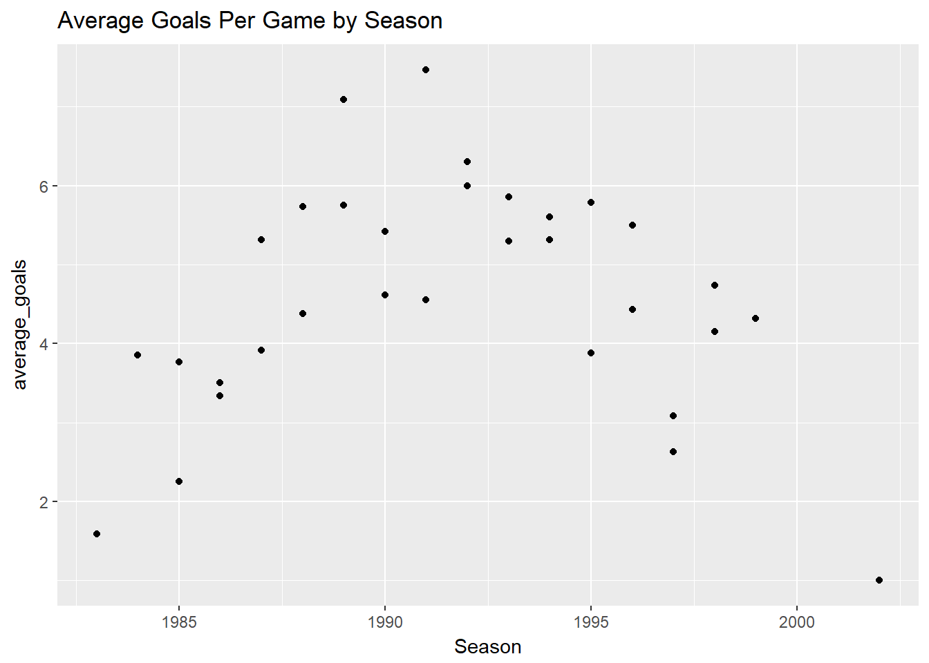
Differentiating the data
One way to differentiate the data is by colour, i.e. we could just colour Tony Lockett one colour and Jason Dunstall another.
df%>%
    select(Season, First.name, Surname, Goals)%>%
    group_by(Season, First.name, Surname)%>%
    summarise(average_goals=mean(Goals))%>%
    filter(First.name %in% c("Tony", "Jason") , Surname %in% c("Lockett", "Dunstall"))%>%
    ggplot(aes(x=Season, y=average_goals)) +
    geom_point(aes(colour=Surname)) +
    ggtitle("Average Goals Per Game by Season")
## Adding missing grouping variables: `Round`, `Home.team`, `Away.team`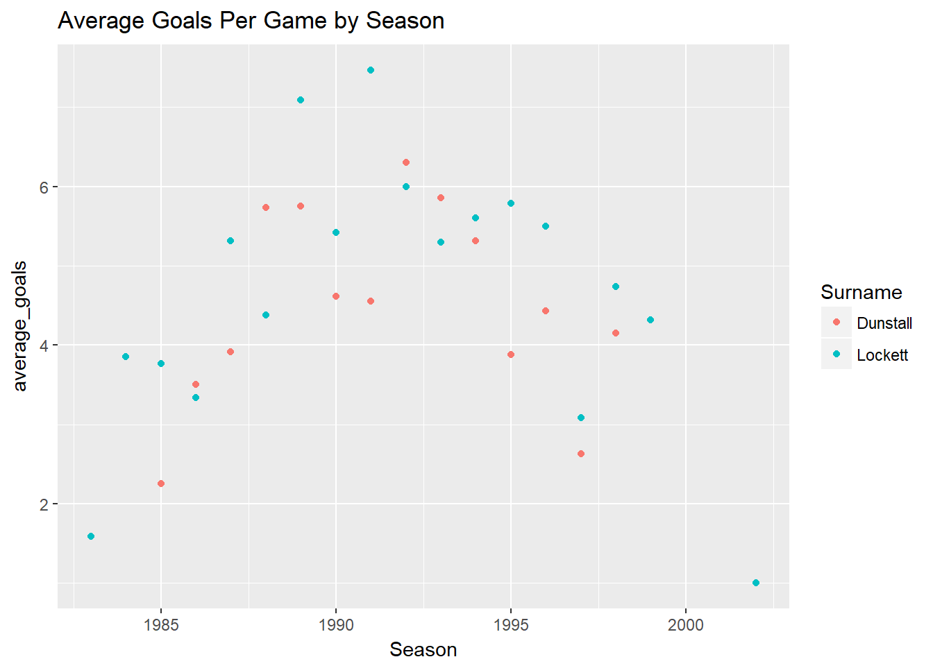
Then we do our line plot like earlier.
df%>%
    select(Season, First.name, Surname, Goals)%>%
    group_by(Season, First.name, Surname)%>%
    summarise(average_goals=mean(Goals))%>%
    filter(First.name %in% c("Tony", "Jason") , Surname %in% c("Lockett", "Dunstall"))%>%
    ggplot(aes(x=Season, y=average_goals)) +
    geom_line(aes(colour=Surname)) +
    ggtitle("Average Goals Per Game by Season")
## Adding missing grouping variables: `Round`, `Home.team`, `Away.team`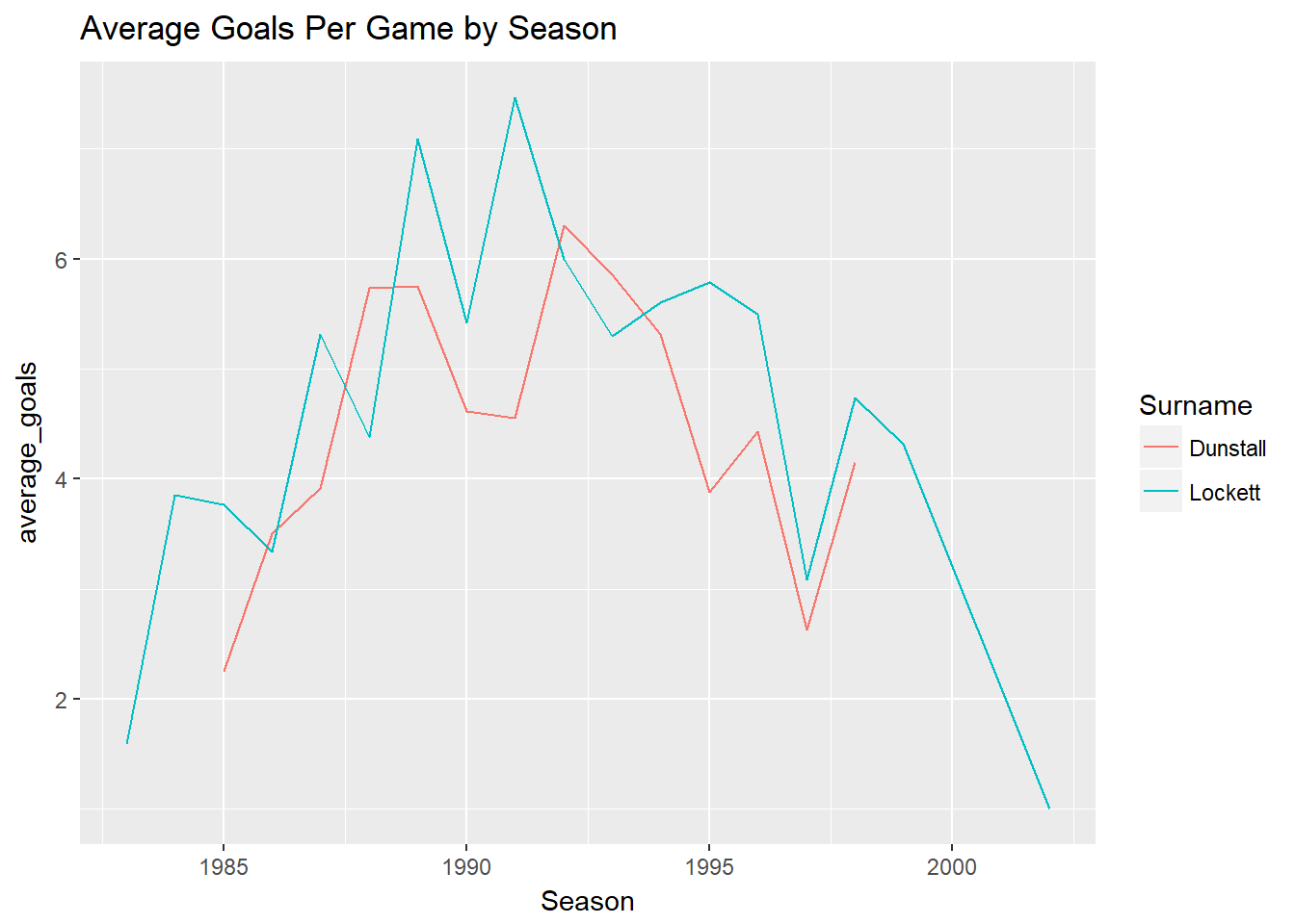
Another way we could plot them, is have the same graph but instead of both lines on one, we could have them side by side for comparison. This is handy in situations where you want to compare the same thing average goals per game by season
This is called small multiples, we do this by using facet_wrap()
df%>%
    select(Season, First.name, Surname, Goals)%>%
    group_by(Season, First.name, Surname)%>%
    summarise(average_goals=mean(Goals))%>%
    filter(First.name %in% c("Tony", "Jason") , Surname %in% c("Lockett", "Dunstall"))%>%
    ggplot(aes(x=Season, y=average_goals)) +
    geom_line() + facet_wrap(~Surname) +
    ggtitle("Average Goals Per Game by Season")
## Adding missing grouping variables: `Round`, `Home.team`, `Away.team`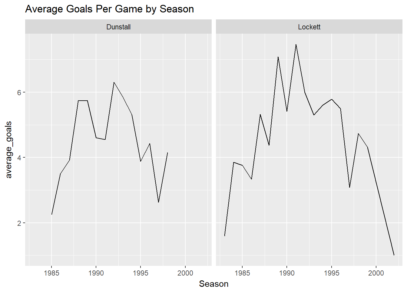
Bonus - You did things in a bad way that might lead to problems
Yes I did, my filter would have taken any unique combinations of First.name , Surname for example if there was a Tony Dunstall or a Jason Lockett they would have come through in the filter.
We can see this if we changed Dunstall to Smith.
df%>%
    select(Season, First.name, Surname, Goals)%>%
    group_by(Season, First.name, Surname)%>%
    summarise(average_goals=mean(Goals))%>%
    filter(First.name %in% c("Tony", "Jason") , Surname %in% c("Lockett", "Smith"))
## Adding missing grouping variables: `Round`, `Home.team`, `Away.team`## # A tibble: 23 x 4
## # Groups: Season, First.name [20]
## Season First.name Surname average_goals
## <dbl> <chr> <chr> <dbl>
## 1 1974 Tony Smith 0
## 2 1983 Tony Lockett 1.58
## 3 1984 Tony Lockett 3.85
## 4 1985 Tony Lockett 3.76
## 5 1986 Tony Lockett 3.33
## 6 1986 Tony Smith 0
## 7 1987 Tony Lockett 5.32
## 8 1987 Tony Smith 0
## 9 1988 Tony Lockett 4.38
## 10 1988 Tony Smith 0.1
## # ... with 13 more rowsSo the best way would be if we had some sort of ID variable. Which luckily in df we have an ID column.
df%>%
    select(Season, First.name, Surname,ID, Goals)%>%
    group_by(Season, First.name, Surname, ID)%>%
    summarise(average_goals=mean(Goals))%>%
    filter(First.name %in% c("Tony", "Jason") , Surname %in% c("Lockett", "Dunstall"))
## Adding missing grouping variables: `Round`, `Home.team`, `Away.team`## # A tibble: 32 x 5
## # Groups: Season, First.name, Surname [32]
## Season First.name Surname ID average_goals
## <dbl> <chr> <chr> <int> <dbl>
## 1 1983 Tony Lockett 990 1.58
## 2 1984 Tony Lockett 990 3.85
## 3 1985 Jason Dunstall 632 2.25
## 4 1985 Tony Lockett 990 3.76
## 5 1986 Jason Dunstall 632 3.5
## 6 1986 Tony Lockett 990 3.33
## 7 1987 Jason Dunstall 632 3.92
## 8 1987 Tony Lockett 990 5.32
## 9 1988 Jason Dunstall 632 5.74
## 10 1988 Tony Lockett 990 4.38
## # ... with 22 more rowsNow we can see our players have the ID of 990 for Lockett and 632 for Dunstall.
So instead of filtering by First.name and Surname we can use the ID instead.
df%>%
    select(Season, First.name, Surname,ID, Goals)%>%
    group_by(Season, First.name, Surname, ID)%>%
    summarise(average_goals=mean(Goals))%>%
    filter(ID %in% c(990,632))
## Adding missing grouping variables: `Round`, `Home.team`, `Away.team`## # A tibble: 32 x 5
## # Groups: Season, First.name, Surname [32]
## Season First.name Surname ID average_goals
## <dbl> <chr> <chr> <int> <dbl>
## 1 1983 Tony Lockett 990 1.58
## 2 1984 Tony Lockett 990 3.85
## 3 1985 Jason Dunstall 632 2.25
## 4 1985 Tony Lockett 990 3.76
## 5 1986 Jason Dunstall 632 3.5
## 6 1986 Tony Lockett 990 3.33
## 7 1987 Jason Dunstall 632 3.92
## 8 1987 Tony Lockett 990 5.32
## 9 1988 Jason Dunstall 632 5.74
## 10 1988 Tony Lockett 990 4.38
## # ... with 22 more rowsThen we can now do our same plots as earlier.
df%>%
    select(Season, First.name, Surname,ID, Goals)%>%
    group_by(Season, First.name, Surname, ID)%>%
    summarise(average_goals=mean(Goals))%>%
    filter(ID %in% c(990,632))%>%
    ggplot(aes(x=Season, y=average_goals)) +
    geom_line() + facet_wrap(~Surname) +
    ggtitle("Average Goals Per Game by Season")
## Adding missing grouping variables: `Round`, `Home.team`, `Away.team`
df%>%
    select(Season, First.name, Surname,ID, Goals)%>%
    group_by(Season, First.name, Surname, ID)%>%
    summarise(average_goals=mean(Goals))%>%
    filter(ID %in% c(990,632))%>%
    ggplot(aes(x=Season, y=average_goals)) +
    geom_line(aes(colour=Surname)) +
    ggtitle("Average Goals Per Game by Season")
## Adding missing grouping variables: `Round`, `Home.team`, `Away.team`