As some of you may be aware, this is the best time of year. Not only is it finals time but its also Brownlow week. During my honours year my thesis was on trying to predict who would win that years Brownlow medal. I have been running the model ever since.
So instead of just giving a list of my predictions for this years count, this post is that will hopefully encourage you at home to give it a go yourself and in doing so you will learn a bit of R and a bit of stats and really what is better than that!
I have uploaded the data that I personally use for my own predictions here
First thing is first, lets read the data in and view it
library(tidyr)
library(ggplot2)
library(dplyr)
library(readr)
library(gapminder)
library(gridExtra)
library(lubridate)
library(dplyr)
library(readxl)
library(aod)
library(ggplot2)
library(knitr)
library(ordinal)
getwd() #make sure the brownlow_data.csv file is saved here
brownlow_data <- read.csv("brownlow_data.csv")
View(brownlow_data)
glimpse(brownlow_data)## Observations: 26,092
## Variables: 40
## $ year <int> 2015, 2015, 2015, 2015, 2015, 2015, 201...
## $ matchId <int> 5964, 5964, 5964, 5964, 5964, 5964, 596...
## $ Round <int> 1, 1, 1, 1, 1, 1, 1, 1, 1, 1, 1, 1, 1, ...
## $ TeamName <fct> Richmond, Carlton, Richmond, Carlton, C...
## $ playerName <fct> Steven Morris, Dale Thomas, Nathan Gord...
## $ kicks <int> 0, 1, 3, 4, 4, 4, 4, 5, 6, 6, 6, 6, 6, ...
## $ handballs <int> 3, 0, 2, 2, 4, 7, 10, 0, 1, 3, 3, 11, 1...
## $ disposals <int> 3, 1, 5, 6, 8, 11, 14, 5, 7, 9, 9, 17, ...
## $ marks <int> 1, 0, 1, 1, 2, 1, 3, 5, 1, 5, 3, 3, 4, ...
## $ hitouts <int> 0, 0, 0, 0, 0, 0, 1, 0, 0, 0, 5, 0, 0, ...
## $ freesFor <int> 1, 1, 1, 1, 0, 1, 0, 0, 2, 0, 1, 0, 1, ...
## $ freesAgainst <int> 5, 0, 0, 0, 0, 0, 0, 4, 1, 0, 0, 0, 1, ...
## $ tackles <int> 4, 0, 0, 4, 1, 1, 3, 1, 1, 0, 2, 1, 5, ...
## $ goals <int> 0, 0, 1, 2, 0, 0, 0, 1, 0, 1, 2, 0, 0, ...
## $ behinds <int> 0, 0, 0, 1, 0, 0, 0, 0, 0, 0, 0, 1, 0, ...
## $ contestedPossessions <int> 2, 1, 1, 4, 3, 7, 5, 1, 3, 0, 4, 5, 10,...
## $ uncontestedPossessions <int> 2, 0, 4, 1, 5, 3, 9, 4, 4, 9, 5, 12, 10...
## $ disposalEfficiency <dbl> 100.0, 100.0, 40.0, 83.3, 62.5, 72.7, 6...
## $ effectivedisposals <int> 3, 1, 2, 5, 5, 8, 9, 3, 6, 9, 6, 9, 15,...
## $ clangers <int> 5, 0, 2, 1, 1, 2, 0, 4, 2, 0, 1, 0, 2, ...
## $ contestedMarks <int> 0, 0, 0, 1, 0, 0, 1, 1, 0, 0, 0, 0, 1, ...
## $ marksIn50 <int> 0, 0, 0, 1, 0, 0, 0, 1, 0, 0, 1, 1, 0, ...
## $ total.clearances <int> 0, 0, 0, 0, 0, 0, 1, 0, 0, 0, 1, 1, 2, ...
## $ rebound50s <int> 0, 0, 0, 0, 1, 3, 2, 1, 2, 2, 1, 1, 2, ...
## $ inside50s <int> 1, 0, 3, 1, 1, 1, 1, 3, 3, 0, 0, 0, 0, ...
## $ onePercenters <int> 4, 0, 0, 0, 6, 4, 0, 6, 3, 1, 6, 0, 2, ...
## $ bounces <int> 0, 0, 0, 0, 0, 0, 0, 0, 0, 0, 0, 0, 0, ...
## $ goalAssists <int> 0, 0, 0, 0, 0, 0, 0, 0, 0, 0, 0, 1, 0, ...
## $ team.total <int> 103, 75, 103, 75, 75, 103, 75, 75, 103,...
## $ margin <int> 28, -28, 28, -28, -28, 28, -28, -28, 28...
## $ centre.clear <int> 0, 0, 0, 0, 0, 0, 0, 0, 0, 0, 0, 0, 0, ...
## $ stoppage.clear <int> 0, 0, 0, 0, 0, 0, 1, 0, 0, 0, 1, 1, 2, ...
## $ score.involvement <int> 2, 1, 1, 4, 3, 6, 2, 2, 1, 3, 2, 4, 6, ...
## $ metersgained <int> -4, -7, 77, 34, 99, 136, 16, 199, 231, ...
## $ turnover <int> 1, 0, 2, 1, 2, 4, 3, 2, 3, 1, 0, 3, 3, ...
## $ intercepts <int> 1, 0, 1, 1, 4, 8, 1, 0, 2, 0, 2, 1, 6, ...
## $ tacklesin50 <int> 2, 0, 0, 0, 0, 0, 0, 0, 0, 0, 0, 1, 0, ...
## $ SC <int> 11, 4, 23, 49, 30, 34, 54, 28, 26, 45, ...
## $ AF <int> 26, 4, 6, 54, 35, 45, 53, 30, 36, 49, 6...
## $ votes <int> 0, 0, 0, 0, 0, 0, 0, 0, 0, 0, 0, 0, 0, ...From our first glimpse we can see that votes is an integer variable, i.e. it can be any whole number from 1 to infinity, we would much rather it be a factor variable as no one can get 4 votes, 5 votes, 6 votes in a game etc. This also helps out when we explore our data graphically later on.
brownlow_data$votes<-as.factor(brownlow_data$votes)Nuffie ideas
Variable creation is one of the most important part of the model building process. As some might say garbage in garbage out. This is also in my opinion the most fun stage of the model building process. Its where you can try to implement your own mental model of the great game.
In general we want to model what our eyes see. It’s just simply not possible for someone to watch all games and come up with their own 3,2,1 for each game. Even if this was possible what you are trying to predict/model isn’t your own model for who is best on, but what you think the umpires opinion is for best on.
For this case we want a model that can be applied to all games across the home and away season based on what we think is predictive of polling votes.
When Tom Mitchell had over 50 touches against the magpies there was a lot of talk around his impact. Something that some footy fans might believe in a Brownlow sense, that hes not going to poll well because he has a high handball to kick ratio. From the dataset above we don’t have that as a variable. So you at home might like to create it, or any other ratio you might like.
Speaking of variable creation, Ryan Buckland has listed some here. You might like to add some or come up with your own.
brownlow_data$h2kr<-brownlow_data$handballs/brownlow_data$kicks
brownlow_data$gr<-(brownlow_data$clangers - brownlow_data$freesAgainst)/brownlow_data$disposals
brownlow_data$tr<-brownlow_data$tackles /brownlow_data$disposals
brownlow_data$mgp<-brownlow_data$metersgained/brownlow_data$disposals
brownlow_data$sfs<-brownlow_data$score.involvement -brownlow_data$goalAssists- brownlow_data$goals - brownlow_data$behindsglimpse(brownlow_data)## Observations: 26,092
## Variables: 45
## $ year <int> 2015, 2015, 2015, 2015, 2015, 2015, 201...
## $ matchId <int> 5964, 5964, 5964, 5964, 5964, 5964, 596...
## $ Round <int> 1, 1, 1, 1, 1, 1, 1, 1, 1, 1, 1, 1, 1, ...
## $ TeamName <fct> Richmond, Carlton, Richmond, Carlton, C...
## $ playerName <fct> Steven Morris, Dale Thomas, Nathan Gord...
## $ kicks <int> 0, 1, 3, 4, 4, 4, 4, 5, 6, 6, 6, 6, 6, ...
## $ handballs <int> 3, 0, 2, 2, 4, 7, 10, 0, 1, 3, 3, 11, 1...
## $ disposals <int> 3, 1, 5, 6, 8, 11, 14, 5, 7, 9, 9, 17, ...
## $ marks <int> 1, 0, 1, 1, 2, 1, 3, 5, 1, 5, 3, 3, 4, ...
## $ hitouts <int> 0, 0, 0, 0, 0, 0, 1, 0, 0, 0, 5, 0, 0, ...
## $ freesFor <int> 1, 1, 1, 1, 0, 1, 0, 0, 2, 0, 1, 0, 1, ...
## $ freesAgainst <int> 5, 0, 0, 0, 0, 0, 0, 4, 1, 0, 0, 0, 1, ...
## $ tackles <int> 4, 0, 0, 4, 1, 1, 3, 1, 1, 0, 2, 1, 5, ...
## $ goals <int> 0, 0, 1, 2, 0, 0, 0, 1, 0, 1, 2, 0, 0, ...
## $ behinds <int> 0, 0, 0, 1, 0, 0, 0, 0, 0, 0, 0, 1, 0, ...
## $ contestedPossessions <int> 2, 1, 1, 4, 3, 7, 5, 1, 3, 0, 4, 5, 10,...
## $ uncontestedPossessions <int> 2, 0, 4, 1, 5, 3, 9, 4, 4, 9, 5, 12, 10...
## $ disposalEfficiency <dbl> 100.0, 100.0, 40.0, 83.3, 62.5, 72.7, 6...
## $ effectivedisposals <int> 3, 1, 2, 5, 5, 8, 9, 3, 6, 9, 6, 9, 15,...
## $ clangers <int> 5, 0, 2, 1, 1, 2, 0, 4, 2, 0, 1, 0, 2, ...
## $ contestedMarks <int> 0, 0, 0, 1, 0, 0, 1, 1, 0, 0, 0, 0, 1, ...
## $ marksIn50 <int> 0, 0, 0, 1, 0, 0, 0, 1, 0, 0, 1, 1, 0, ...
## $ total.clearances <int> 0, 0, 0, 0, 0, 0, 1, 0, 0, 0, 1, 1, 2, ...
## $ rebound50s <int> 0, 0, 0, 0, 1, 3, 2, 1, 2, 2, 1, 1, 2, ...
## $ inside50s <int> 1, 0, 3, 1, 1, 1, 1, 3, 3, 0, 0, 0, 0, ...
## $ onePercenters <int> 4, 0, 0, 0, 6, 4, 0, 6, 3, 1, 6, 0, 2, ...
## $ bounces <int> 0, 0, 0, 0, 0, 0, 0, 0, 0, 0, 0, 0, 0, ...
## $ goalAssists <int> 0, 0, 0, 0, 0, 0, 0, 0, 0, 0, 0, 1, 0, ...
## $ team.total <int> 103, 75, 103, 75, 75, 103, 75, 75, 103,...
## $ margin <int> 28, -28, 28, -28, -28, 28, -28, -28, 28...
## $ centre.clear <int> 0, 0, 0, 0, 0, 0, 0, 0, 0, 0, 0, 0, 0, ...
## $ stoppage.clear <int> 0, 0, 0, 0, 0, 0, 1, 0, 0, 0, 1, 1, 2, ...
## $ score.involvement <int> 2, 1, 1, 4, 3, 6, 2, 2, 1, 3, 2, 4, 6, ...
## $ metersgained <int> -4, -7, 77, 34, 99, 136, 16, 199, 231, ...
## $ turnover <int> 1, 0, 2, 1, 2, 4, 3, 2, 3, 1, 0, 3, 3, ...
## $ intercepts <int> 1, 0, 1, 1, 4, 8, 1, 0, 2, 0, 2, 1, 6, ...
## $ tacklesin50 <int> 2, 0, 0, 0, 0, 0, 0, 0, 0, 0, 0, 1, 0, ...
## $ SC <int> 11, 4, 23, 49, 30, 34, 54, 28, 26, 45, ...
## $ AF <int> 26, 4, 6, 54, 35, 45, 53, 30, 36, 49, 6...
## $ votes <fct> 0, 0, 0, 0, 0, 0, 0, 0, 0, 0, 0, 0, 0, ...
## $ h2kr <dbl> Inf, 0.0000000, 0.6666667, 0.5000000, 1...
## $ gr <dbl> 0.00000000, 0.00000000, 0.40000000, 0.1...
## $ tr <dbl> 1.33333333, 0.00000000, 0.00000000, 0.6...
## $ mgp <dbl> -1.333333, -7.000000, 15.400000, 5.6666...
## $ sfs <int> 2, 1, 0, 1, 3, 6, 2, 1, 1, 2, 0, 2, 6, ...After creating a list of your own variables you want to give them a look what you will notice is that there will be some infinate values and NaN values. We can just replace them with 0.
 is.na(brownlow_data)<-sapply(brownlow_data, is.infinite)
 brownlow_data[is.na(brownlow_data)]<-0
 glimpse(brownlow_data)
## Observations: 26,092
## Variables: 45
## $ year <int> 2015, 2015, 2015, 2015, 2015, 2015, 201...
## $ matchId <int> 5964, 5964, 5964, 5964, 5964, 5964, 596...
## $ Round <int> 1, 1, 1, 1, 1, 1, 1, 1, 1, 1, 1, 1, 1, ...
## $ TeamName <fct> Richmond, Carlton, Richmond, Carlton, C...
## $ playerName <fct> Steven Morris, Dale Thomas, Nathan Gord...
## $ kicks <int> 0, 1, 3, 4, 4, 4, 4, 5, 6, 6, 6, 6, 6, ...
## $ handballs <int> 3, 0, 2, 2, 4, 7, 10, 0, 1, 3, 3, 11, 1...
## $ disposals <int> 3, 1, 5, 6, 8, 11, 14, 5, 7, 9, 9, 17, ...
## $ marks <int> 1, 0, 1, 1, 2, 1, 3, 5, 1, 5, 3, 3, 4, ...
## $ hitouts <int> 0, 0, 0, 0, 0, 0, 1, 0, 0, 0, 5, 0, 0, ...
## $ freesFor <int> 1, 1, 1, 1, 0, 1, 0, 0, 2, 0, 1, 0, 1, ...
## $ freesAgainst <int> 5, 0, 0, 0, 0, 0, 0, 4, 1, 0, 0, 0, 1, ...
## $ tackles <int> 4, 0, 0, 4, 1, 1, 3, 1, 1, 0, 2, 1, 5, ...
## $ goals <int> 0, 0, 1, 2, 0, 0, 0, 1, 0, 1, 2, 0, 0, ...
## $ behinds <int> 0, 0, 0, 1, 0, 0, 0, 0, 0, 0, 0, 1, 0, ...
## $ contestedPossessions <int> 2, 1, 1, 4, 3, 7, 5, 1, 3, 0, 4, 5, 10,...
## $ uncontestedPossessions <int> 2, 0, 4, 1, 5, 3, 9, 4, 4, 9, 5, 12, 10...
## $ disposalEfficiency <dbl> 100.0, 100.0, 40.0, 83.3, 62.5, 72.7, 6...
## $ effectivedisposals <int> 3, 1, 2, 5, 5, 8, 9, 3, 6, 9, 6, 9, 15,...
## $ clangers <int> 5, 0, 2, 1, 1, 2, 0, 4, 2, 0, 1, 0, 2, ...
## $ contestedMarks <int> 0, 0, 0, 1, 0, 0, 1, 1, 0, 0, 0, 0, 1, ...
## $ marksIn50 <int> 0, 0, 0, 1, 0, 0, 0, 1, 0, 0, 1, 1, 0, ...
## $ total.clearances <int> 0, 0, 0, 0, 0, 0, 1, 0, 0, 0, 1, 1, 2, ...
## $ rebound50s <int> 0, 0, 0, 0, 1, 3, 2, 1, 2, 2, 1, 1, 2, ...
## $ inside50s <int> 1, 0, 3, 1, 1, 1, 1, 3, 3, 0, 0, 0, 0, ...
## $ onePercenters <int> 4, 0, 0, 0, 6, 4, 0, 6, 3, 1, 6, 0, 2, ...
## $ bounces <int> 0, 0, 0, 0, 0, 0, 0, 0, 0, 0, 0, 0, 0, ...
## $ goalAssists <int> 0, 0, 0, 0, 0, 0, 0, 0, 0, 0, 0, 1, 0, ...
## $ team.total <int> 103, 75, 103, 75, 75, 103, 75, 75, 103,...
## $ margin <int> 28, -28, 28, -28, -28, 28, -28, -28, 28...
## $ centre.clear <int> 0, 0, 0, 0, 0, 0, 0, 0, 0, 0, 0, 0, 0, ...
## $ stoppage.clear <int> 0, 0, 0, 0, 0, 0, 1, 0, 0, 0, 1, 1, 2, ...
## $ score.involvement <int> 2, 1, 1, 4, 3, 6, 2, 2, 1, 3, 2, 4, 6, ...
## $ metersgained <int> -4, -7, 77, 34, 99, 136, 16, 199, 231, ...
## $ turnover <int> 1, 0, 2, 1, 2, 4, 3, 2, 3, 1, 0, 3, 3, ...
## $ intercepts <int> 1, 0, 1, 1, 4, 8, 1, 0, 2, 0, 2, 1, 6, ...
## $ tacklesin50 <int> 2, 0, 0, 0, 0, 0, 0, 0, 0, 0, 0, 1, 0, ...
## $ SC <int> 11, 4, 23, 49, 30, 34, 54, 28, 26, 45, ...
## $ AF <int> 26, 4, 6, 54, 35, 45, 53, 30, 36, 49, 6...
## $ votes <fct> 0, 0, 0, 0, 0, 0, 0, 0, 0, 0, 0, 0, 0, ...
## $ h2kr <dbl> 0.0000000, 0.0000000, 0.6666667, 0.5000...
## $ gr <dbl> 0.00000000, 0.00000000, 0.40000000, 0.1...
## $ tr <dbl> 1.33333333, 0.00000000, 0.00000000, 0.6...
## $ mgp <dbl> -1.333333, -7.000000, 15.400000, 5.6666...
## $ sfs <int> 2, 1, 0, 1, 3, 6, 2, 1, 1, 2, 0, 2, 6, ...Plot your data
‘The simple graph has brought more information to the data analysts mind than any other device.’ John Tukey
So now you have your data and its nicely organised, lets do some plotting!
One of my personal favourite graphs for comparisons between groups is the boxplot
What we are looking for is for variables where the ‘box’ part is increasing as you go from 0 vote category to the 3 vote category.
As an example of increasing ‘boxes’ lets look at SC which is the supercoach score of the player in the game.
p <- ggplot(brownlow_data, aes(votes, SC))
p + geom_boxplot() + ggtitle("Supercoach Scores Vs Brownlow Votes") +ylab("Supercoach Score")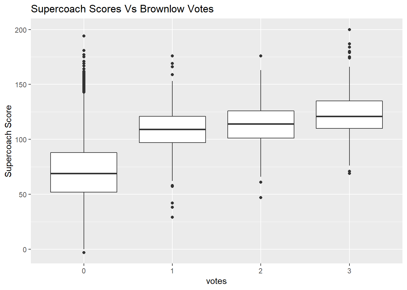
So looking at that graph, it would seem as though it makes sense to include Supercoach scores as a predictor in your own Brownlow Model.
Lets look at a variable that doesn’t seem to seperate players into voting categories.
p <- ggplot(brownlow_data, aes(votes, gr))
p + geom_boxplot() 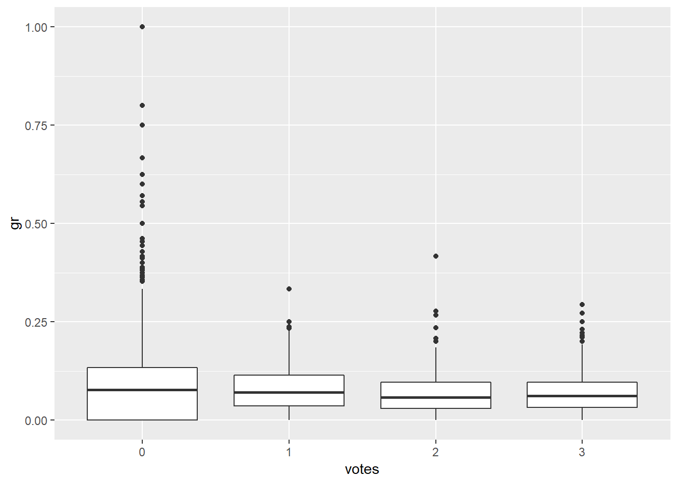 After exploring the variables you yourself will come up with a list of variables that you think are predictive they might be stats that are already being provided or you might be creative and create some of your own.
Whatever the case maybe lets put those variables in a model!
The model
The model below is an ordinal regression model. Ordinal because there is some natural ordering to do with the voting categories. A player who gets 3 votes should have better in game statistics over a player who didn’t poll. This method is commonly used in medical sciences such as prediction of a patient conditions. In this case the ordering could be considered healthy, servere, dying. The CLM package in R is used to fit such models.
In our script below this will involve a few steps
Create our dataset for modelling : This will involve selecting the variables we think might be predictive of polling well in the 2017 Brownlow Medal
Standardising our data : for why we standardise a good read is here
- Using the CLM package we create our model which has votes as our outcome variable and our 6 predictors are
- disposals
- contestedPossessions
- score.involvement
- SC (Supercoach scores)
- intercepts
- sfs (Score Facilitation Score)
- mgp (Metres Gained per Disposal)
- Apply that model to 2017 dataset to get the predicted probabilities that a player will poll 3 votes
*p3, 2 votes*p2, 1 vote*p1and no votesp0 - Come up with the expected votes for each player in a game
expected_votes= 0*p0+1*p1+2*p2+3*p3
- sum up the expected votes for the year for each player to form our predicted order.
#create our dataset for modelling

dataR<-select(brownlow_data, #base dataset
              year, matchId, Round, TeamName, playerName, #variables that you want for filtering
              disposals, contestedPossessions,score.involvement,SC,intercepts,sfs,mgp,votes #variables that seem predictive?
)

in.sample  <- subset(dataR, year %in% c(2015:2016)) #our traning data

out.sample <- subset(dataR, year == 2017) #the prediction year

temp1<-scale(in.sample[,6:12]) #I am standardising the 6th column (disposals) until the 12th column (mgp)
in.sample[,6:12]<-temp1
# attributes(temp1)
temp1.center<-attr(temp1,"scaled:center")
temp1.scale<-attr(temp1,"scaled:scale")

fm1<-clm(votes~ disposals +contestedPossessions+score.involvement+SC+intercepts+sfs +mgp,
         data = in.sample)
summary(fm1)
## formula:
## votes ~ disposals + contestedPossessions + score.involvement + SC + intercepts + sfs + mgp
## data: in.sample
##
## link threshold nobs logLik AIC niter max.grad cond.H
## logit flexible 17380 -3495.58 7011.16 9(1) 2.77e-13 1.8e+02
##
## Coefficients:
## Estimate Std. Error z value Pr(>|z|)
## disposals 0.43325 0.06777 6.393 1.62e-10 ***
## contestedPossessions 0.50887 0.03977 12.795 < 2e-16 ***
## score.involvement 1.06931 0.05742 18.623 < 2e-16 ***
## SC 1.41717 0.07005 20.230 < 2e-16 ***
## intercepts 0.03264 0.04075 0.801 0.423
## sfs -0.58335 0.05405 -10.793 < 2e-16 ***
## mgp 0.23567 0.05069 4.649 3.34e-06 ***
## ---
## Signif. codes: 0 '***' 0.001 '**' 0.01 '*' 0.05 '.' 0.1 ' ' 1
##
## Threshold coefficients:
## Estimate Std. Error z value
## 0|1 4.81999 0.08600 56.05
## 1|2 5.51674 0.09484 58.17
## 2|3 6.57763 0.11055 59.50newdata <- out.sample[ , -ncol(out.sample)]
newdata[,6:12]<-scale(newdata[,6:12],center=temp1.center,scale=temp1.scale)
pre.dict <- predict(fm1,newdata=newdata, type='prob')
pre.dict.m <- data.frame(matrix(unlist(pre.dict), nrow= nrow(newdata)))
colnames(pre.dict.m) <- c("vote.0", "vote.1", "vote.2", "vote.3")
newdata.pred <- cbind.data.frame(newdata, pre.dict.m)
### Step 1: Get expected value on Votes
newdata.pred$expected.votes <- newdata.pred$vote.1 + 2*newdata.pred$vote.2 + 3*newdata.pred$vote.3
prediction <- aggregate(expected.votes~playerName, data = newdata.pred, FUN = sum )
predicted_order <- arrange(prediction,desc(expected.votes)) #making an ordered tablekable(predicted_order[1:10, ], caption = "Your top 10.")| playerName | expected.votes |
|---|---|
| Patrick Dangerfield | 35.74528 |
| Dustin Martin | 29.58564 |
| Tom Mitchell | 28.03692 |
| Rory Sloane | 24.55525 |
| Dayne Zorko | 24.28554 |
| Joshua Kelly | 17.90181 |
| Dayne Beams | 17.76031 |
| Gary Jnr Ablett | 17.16746 |
| Lance Franklin | 17.11848 |
| Taylor Adams | 17.11708 |
So there you go, based on this simple six variable model, Patrick Dangerfield after being shockingly suspended will poll the most votes but hand over his medal to Dusty.